
Attention in Neural Networks - 11. Alignment Models (4)
16 Mar 2020 | Attention mechanism Deep learning PytorchAttention Mechanism in Neural Networks - 11. Alignment Models (4)
So far, we reviewed and implemented the Seq2Seq model with alignment proposed by Bahdahanu et al. (2015). In this posting, let’s try mini-batch training and evaluation of the model as we did for the vanilla Seq2Seq in this posting
Import and process data
This part is identical to what we did for mini-batch training of the vanilla Seq2Seq. So, I will let you refer to the posting to save space.
Setting parameters
Seting parameters are also identical. For the purpose of sanity check, the parameters can be set to as below.
ENG_VOCAB_SIZE = len(eng_words)
DEU_VOCAB_SIZE = len(deu_words)
LEARNING_RATE = 1e-2
NUM_EPOCHS = 10
HIDDEN_SIZE = 128
EMBEDDING_DIM = 30
DEVICE = torch.device('cuda')
Encoder and Decoder
Similarly, we define the encoder and decoder separately and merge them in the Seq2Seq model. The encoder is defined similarly to the original model, so the emphasis is on the decoder here. Note how the training data is sliced to fit into the decoder model that processes mini-batch inputs.
class Encoder(nn.Module):
  def __init__(self, vocab_size, hidden_size, max_sent_len, embedding_dim):
    super(Encoder, self).__init__()
    self.hidden_size = hidden_size
    self.max_sent_len = max_sent_len

    self.embedding = nn.Embedding(vocab_size, embedding_dim)
    self.gru = nn.GRU(embedding_dim, hidden_size)

  def forward(self, source):
    source = self.embedding(source)
    enc_outputs = torch.zeros(self.max_sent_len, source.size(0), self.hidden_size).to(DEVICE)
    h0 = torch.zeros(1, source.size(0), self.hidden_size).to(DEVICE)  # encoder hidden state = (1, BATCH_SIZE, HIDDEN_SIZE)
    for k in range(source.size(1)):
      _, h0 = self.gru(source[:, k].unsqueeze(0), h0)
      enc_outputs[k, :] = h0.squeeze()
    return enc_outputs

class Decoder(nn.Module):
  def __init__(self, vocab_size, hidden_size, embedding_dim, device):
    super(Decoder, self).__init__()
    self.hidden_size = hidden_size
    self.device = device
    self.vocab_size = vocab_size

    self.embedding = nn.Embedding(vocab_size, embedding_dim)
    self.attention = nn.Linear(hidden_size + hidden_size, 1)
    self.gru = nn.GRU(hidden_size + embedding_dim, hidden_size)
    self.dense = nn.Linear(hidden_size, vocab_size)
    self.softmax = nn.Softmax(dim=1)
    self.log_softmax = nn.LogSoftmax(dim = 1)
    self.relu = nn.ReLU()

  def forward(self, decoder_input, current_hidden_state, encoder_outputs):

    decoder_input = self.embedding(decoder_input)    # (BATCH_SIZE, EMBEDDING_DIM)
    aligned_weights = torch.randn(encoder_outputs.size(0), encoder_outputs.size(1)).to(self.device)

    for i in range(encoder_outputs.size(0)):
      aligned_weights[i] = self.attention(torch.cat((current_hidden_state, encoder_outputs[i].unsqueeze(0)), dim = -1)).squeeze()

    aligned_weights = self.softmax(aligned_weights)   # (BATCH_SIZE, HIDDEN_STATE * 2)
    aligned_weights = aligned_weights.view(aligned_weights.size(1), aligned_weights.size(0))

    context_vector = torch.bmm(aligned_weights.unsqueeze(1), encoder_outputs.view(encoder_outputs.size(1), encoder_outputs.size(0), encoder_outputs.size(2)))

    x = torch.cat((context_vector.squeeze(1), decoder_input), dim = 1).unsqueeze(0)
    x = self.relu(x)
    x, current_hidden_state = self.gru(x, current_hidden_state)
    x = self.log_softmax(self.dense(x.squeeze(0)))
    return x, current_hidden_state, aligned_weights
Seq2Seq model
Now we merge the encoder and decoder to create a Seq2Seq model. Since we have already defined the encoder and decoder in detail, implementing the Seq2Seq model is straightforward. Just notice how the hidden states of decoder (dec_h0) and weights (w) are updated at each step.
class AttenS2S(nn.Module):
  def __init__(self, encoder, decoder, max_sent_len, device):
    super(AttenS2S, self).__init__()
    self.encoder = encoder
    self.decoder = decoder
    self.device = device
    self.max_sent_len = max_sent_len

  def forward(self, source, target, tf_ratio = .5):
    enc_outputs = self.encoder(source)
    dec_outputs = torch.zeros(target.size(0), target.size(1), self.decoder.vocab_size).to(self.device)
    dec_input = target[:, 0]
    dec_h0 = torch.zeros(1, dec_input.size(0), self.encoder.hidden_size).to(DEVICE)
    weights = torch.zeros(target.size(1), target.size(0), target.size(1))   # (TARGET_LEN, BATCH_SIZE, SOURCE_LEN)
    for k in range(target.size(1)):
      out, dec_h0, w = self.decoder(dec_input, dec_h0, enc_outputs)
      weights[k, :, :] = w
      dec_outputs[:, k] = out
      if np.random.choice([True, False], p = [tf_ratio, 1-tf_ratio]):
        dec_input = target[:, k]
      else:
        dec_input = out.argmax(1).detach()

    return dec_outputs, weights
Training
Training is also done in a similar fashion. Just be aware of calculating the negative log likelihood loss. The output has one more dimension, i.e., batch size, so it needs to be reshaped to collapse into two dimensions to calculate the loss.
encoder = Encoder(ENG_VOCAB_SIZE, HIDDEN_SIZE, MAX_SENT_LEN, EMBEDDING_DIM).to(DEVICE)
decoder = Decoder(DEU_VOCAB_SIZE, HIDDEN_SIZE, EMBEDDING_DIM, DEVICE).to(DEVICE)
seq2seq = AttenS2S(encoder, decoder, MAX_SENT_LEN, DEVICE).to(DEVICE)
criterion = nn.NLLLoss()
optimizer = torch.optim.Adam(seq2seq.parameters(), lr = LEARNING_RATE)

%%time
loss_trace = []
for epoch in tqdm(range(NUM_EPOCHS)):
  current_loss = 0
  for i, (x, y) in enumerate(train_loader):
    x, y  = x.to(DEVICE), y.to(DEVICE)
    outputs, _ = seq2seq(x, y)
    loss = criterion(outputs.resize(outputs.size(0) * outputs.size(1), outputs.size(-1)), y.resize(y.size(0) * y.size(1)))
    optimizer.zero_grad()
    loss.backward()
    optimizer.step()
    current_loss += loss.item()
  loss_trace.append(current_loss)
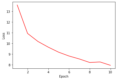
Let’s try visualizing the loss trace with a plot. The loss continually decreases up to the 10th epoch. Please try training over 10 epochs for more effective training.
# loss curve
plt.plot(range(1, NUM_EPOCHS+1), loss_trace, 'r-')
plt.xlabel('Epoch')
plt.ylabel('Loss')
plt.show()
Evaluation and visualization
In mini-batch implementation of alignment models, learned weights need to be permuted as there is another dimension here as well.
%%time
test_weights = []
source, target = [], []
for i, (x, y) in enumerate(test_loader):
  with torch.no_grad():
    for s in x:
      source.append(s.detach().cpu().numpy())
    for t in y:
      target.append(t.detach().cpu().numpy())
    x, y  = x.to(DEVICE), y.to(DEVICE)
    outputs, current_weights = seq2seq(x, y)
    current_weights = current_weights.permute(1, 0, 2)
    for cw in current_weights:
      test_weights.append(cw.detach().cpu().numpy())
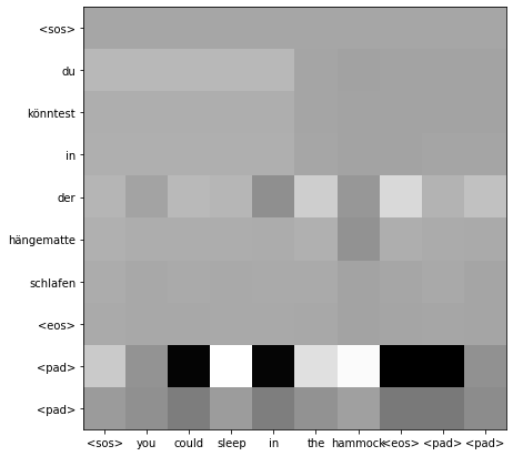
And each weight can be visualized using a matplotlib heatmap. Below is an example of visualizing the learned weights of the second test instance according to their saliency.
idx = 1

source_sent = [eng_words[x] for x in source[idx]]
target_sent = [deu_words[x] for x in target[idx]]

fig, ax = plt.subplots(figsize = (7,7))
im = ax.imshow(test_weights[idx], cmap = "binary")
ax.set_xticks(np.arange(len(source_sent)))
ax.set_yticks(np.arange(len(target_sent)))
ax.set_xticklabels(source_sent)
ax.set_yticklabels(target_sent)
plt.show()
In this posting, we implemented mini-batch alignment Seq2Seq proposed by Bahdahanu et al. (2015). In the following postings, let’s look into various types of attentional models beyond the Bahdanau attention. Thank you for reading.