Attention Mechanism in Neural Networks - 12. Various attention mechanisms (1)

In a few recent postings, we looked into the attention mechanism for aligning source and target sentences in machine translation proposed by Bahdahanu et al. (2015). However, there are a number of attention functions such as those outlined in here. From now on, let’s dig into various attention methods outlined by Luong et al. (2015)

Global and Local attention - where the attention is applied

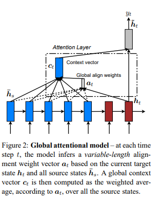
First, Luong et al. distinguishes global and local attention. Both have a common goal of estimating the context vector $c_t$ and the probability of the target word $p(y_t)$ at each timestep of $t$. However, two differs in where the attention is applied among timesteps in the encoder. Global attention is similar to what we have looked into in previous postings. It considers all hidden states of encoder ($h_t$) and aligns them with current decoder input.

In contrast, local attention focuses on a small window of context and aligns source states in such window. By doing so, it is less computationally expensive and easier to train. It is a blend of hard and soft attention proposed by Xu et al. (2015)

“Our local attention mechanism selectively focuses on a small window of context and is differentiable. This approach has an advantage of avoiding the expensive computation incurred in the soft attention and at the same time, is easier to train than the hard attention approach.”

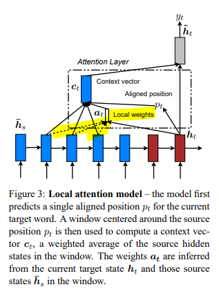
Thus, there is an additional step of alignment in local attention - i.e., searching for an aligned position $p_t$ for each target word at timestep $t$. Then, the context vector $c_t$ is similarly estimated to global attention but applied only to the context window of $[p_t - D, p_t + D]$. $D$ can be empirically selected by the developer. In other words, attention is applied to the local context of $2D+1$ timesteps.

Searching for aligned position

Two methods for estimating the aligned position are suggested by Luong et al. (2015) - (1) monotonic alignment (local-m) and (2) predictive alignment (local-p). Monotonic alignment simply sets $p_t = t$. The intuition behind local-m is that source and target sequences are, at least roughly, aligned in a monotonous fashion. Whereas predictive alignment “predicts” each $p_t$ with below function. $W_p$ and $v_p$ are model parameters that are trained and $S$ is the length of a source sentence.

\begin{equation} p_t = S \cdot sigmoid(v_p^{T}tanh(W_ph_t)) \end{equation}

Scoring functions - how to measure the similarity between inputs

Prior to estimating the context vector $c_t$, the (local or global) alignment weights $\alpha_t$ should be learned. $\alpha_t$ at each timestep of $s$ in source sentence can be calculated as below. $\bar{h_s}$ is the source hidden state at timestep $s$.

\begin{equation} \alpha_t(s) = \frac{exp(score(h_t, \bar{h_s}))}{\sum_{s’}exp(score(h_t, \bar{h_{s’}}))} \end{equation}

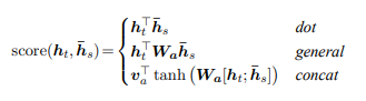
There are a variety of scoring functions, i.e., $score()$, . Three functions that are proposed by Luong et al. (2015) are dot, general, and concat functions. The intuition behind different types of scoring functions is similar to that of cosine similarity. In the cosine similarity function, dot product basically estimates similarity between two inputs. Similarly, scoring functions calculate similarity between the source and target hidden states.

In this posting, we closely looked into various attention mechanisms proposed by Luong et al. (2015). In the following postings, let’s see how they can be implemented with Pytorch. Thank you for reading.

References

• Luong et al. (2015)