Attention in Neural Networks - 19. Transformer (3)
21 Apr 2020 | Attention mechanism Deep learning PytorchAttention Mechanism in Neural Networks - 19. Transformer (3)
In the previous posting, we tried implementing the simple Transformer architecture with nn.Transformer. In this posting, let’s dig a little deeper and see how nn.Transformer works under the hood.
Data import & preprocessing
Steps up to creating dataset and datalodaer are almost identical. So you can skim through these preliminary steps if you are familar with.
Using Jupyter Notebook or Google Colaboratory, the data file can be fetched directly from the Web and unzipped.
!wget https://www.manythings.org/anki/deu-eng.zip
!unzip deu-eng.zip

with open("deu.txt") as f:
  sentences = f.readlines()
As we did before, let’s randomly sample 10,000 instances and process them.
NUM_INSTANCES = 10000
MAX_SENT_LEN = 10
eng_sentences, deu_sentences = [], []
eng_words, deu_words = set(), set()
for i in tqdm(range(NUM_INSTANCES)):
  rand_idx = np.random.randint(len(sentences))
  # find only letters in sentences
  eng_sent, deu_sent = ["<sos>"], ["<sos>"]
  eng_sent += re.findall(r"\w+", sentences[rand_idx].split("\t")[0])
  deu_sent += re.findall(r"\w+", sentences[rand_idx].split("\t")[1])

  # change to lowercase
  eng_sent = [x.lower() for x in eng_sent]
  deu_sent = [x.lower() for x in deu_sent]
  eng_sent.append("<eos>")
  deu_sent.append("<eos>")

  if len(eng_sent) >= MAX_SENT_LEN:
    eng_sent = eng_sent[:MAX_SENT_LEN]
  else:
    for _ in range(MAX_SENT_LEN - len(eng_sent)):
      eng_sent.append("<pad>")

  if len(deu_sent) >= MAX_SENT_LEN:
    deu_sent = deu_sent[:MAX_SENT_LEN]
  else:
    for _ in range(MAX_SENT_LEN - len(deu_sent)):
      deu_sent.append("<pad>")

  # add parsed sentences
  eng_sentences.append(eng_sent)
  deu_sentences.append(deu_sent)

  # update unique words
  eng_words.update(eng_sent)
  deu_words.update(deu_sent)

eng_words, deu_words = list(eng_words), list(deu_words)

# encode each token into index
for i in tqdm(range(len(eng_sentences))):
  eng_sentences[i] = [eng_words.index(x) for x in eng_sentences[i]]
  deu_sentences[i] = [deu_words.index(x) for x in deu_sentences[i]]

idx = 10
print(eng_sentences[idx])
print([eng_words[x] for x in eng_sentences[idx]])
print(deu_sentences[idx])
print([deu_words[x] for x in deu_sentences[idx]])
If properly imported and processed, you will get an output something like this. But specific values of output will be somewhat different since we are randomly sampling instances.
[2142, 1843, 174, 3029, 1716, 3449, 4385, 2021, 4359, 4359]
['<sos>', 'tom', 'didn', 't', 'have', 'a', 'chance', '<eos>', '<pad>', '<pad>']
[2570, 6013, 2486, 2470, 1631, 2524, 3415, 3415, 3415, 3415]
['<sos>', 'tom', 'hatte', 'keine', 'chance', '<eos>', '<pad>', '<pad>', '<pad>', '<pad>']
Setting Parameters
Most of paramter setting is similar to the RNN Encoder-Decoder network and its variants.
HIDDEN SIZE: previously this was used to set the number of hidden cells in the RNN network. However, here it will be used to set the dimensionality of the feedforward network, or the dense layers.NUM_LAYERS: similary, instead of setting the number of RNN layers, this is used to determine the number of dense layers.NUM_HEADS: this is a new parameter used to determine the number of heads in multihead attention. If you are unsure what multihead attention is, refer to the previous posting.DROPOUT: Another parameter that we can consider isDROPOUT, which determines the probability of dropping out a node in the encoder/decoder layer. This can be set to the same value across all layers, or can be fine-tuned to set to different values in each layer. However, in most cases it is a single value across all layers for simplicity.
ENG_VOCAB_SIZE = len(eng_words)
DEU_VOCAB_SIZE = len(deu_words)
NUM_EPOCHS = 10
HIDDEN_SIZE = 16
EMBEDDING_DIM = 30
BATCH_SIZE = 128
NUM_HEADS = 2
NUM_LAYERS = 3
LEARNING_RATE = 1e-2
DROPOUT = .3
DEVICE = torch.device('cuda')
Creating dataset and dataloader
This is exactly the same step as before, so I won’t explain the details. Again, if you want to know more, please refer to the previous postings.
class MTDataset(torch.utils.data.Dataset):
  def __init__(self):
    # import and initialize dataset
    self.source = np.array(eng_sentences, dtype = int)
    self.target = np.array(deu_sentences, dtype = int)

  def __getitem__(self, idx):
    # get item by index
    return self.source[idx], self.target[idx]

  def __len__(self):
    # returns length of data
    return len(self.source)

np.random.seed(777)   # for reproducibility
dataset = MTDataset()
NUM_INSTANCES = len(dataset)
TEST_RATIO = 0.3
TEST_SIZE = int(NUM_INSTANCES * 0.3)

indices = list(range(NUM_INSTANCES))

test_idx = np.random.choice(indices, size = TEST_SIZE, replace = False)
train_idx = list(set(indices) - set(test_idx))
train_sampler, test_sampler = SubsetRandomSampler(train_idx), SubsetRandomSampler(test_idx)

train_loader = torch.utils.data.DataLoader(dataset, batch_size = BATCH_SIZE, sampler = train_sampler)
test_loader = torch.utils.data.DataLoader(dataset, batch_size = BATCH_SIZE, sampler = test_sampler)
Under the hood of nn.Transformer
The best way to understand how Pytorch models work is by analyzing tensor operations between layers and functions. In most cases, we do not need to attend to the specific values of tensors, but just can keep track of tensor shapes, or sizes. Making sense of how each element in the size (shape) array is mapped to dimensionality of input/output tensors and how they are manipulated with matrix operations are critical.
Here, let’s fetch the first batch of the training data and see how it is transformed step-by-step in the Transformer network.
Each batch tensor from the train_loader has the shape of (BATCH_SIZE, MAX_SENT_LEN).
src, tgt = next(iter(train_loader))
print(src.shape, tgt.shape)   # (BATCH_SIZE, SEQ_LEN)
Embedding
After being embedded, they have the shape of (BATCH_SIZE, MAX_SENT_LEN, EMBEDDING_DIM).
enc_embedding = nn.Embedding(ENG_VOCAB_SIZE, EMBEDDING_DIM)
dec_embedding = nn.Embedding(DEU_VOCAB_SIZE, EMBEDDING_DIM)
src, tgt = enc_embedding(src), dec_embedding(tgt)
print(src.shape, tgt.shape)                # (BATCH_SIZE, SEQ_LEN, EMBEDDING_DIM)
Positional encoding
Then, the embedded tensors have to be positionally encoded to take into account the order of sequences. I borrowed this code from the official Pytorch Tranformer tutorial, after just replacing math.log() with np.log().
## source: https://pytorch.org/tutorials/beginner/transformer_tutorial.html
class PositionalEncoding(nn.Module):
    def __init__(self, d_model, dropout=0.1, max_len=5000):
        super(PositionalEncoding, self).__init__()
        self.dropout = nn.Dropout(p=dropout)
        pe = torch.zeros(max_len, d_model)
        position = torch.arange(0, max_len, dtype=torch.float).unsqueeze(1)
        div_term = torch.exp(torch.arange(0, d_model, 2).float() * (-np.log(10000.0) / d_model))
        pe[:, 0::2] = torch.sin(position * div_term)
        pe[:, 1::2] = torch.cos(position * div_term)
        pe = pe.unsqueeze(0).transpose(0, 1)
        self.register_buffer('pe', pe)

    def forward(self, x):
        x = x + self.pe[:x.size(0), :]
        return self.dropout(x)
Before positional encoding, we swap the first and second dimensions. This can be sometimes unnecessary if your data shape is different or employing different code for positional encoding. And after positional encoding, the tensors have the same shape. Remember that positional encoding is simply element-wise adding information regarding the relative/absolute position without altering the tensor shape.
pe = PositionalEncoding(EMBEDDING_DIM, max_len = MAX_SENT_LEN)
src, tgt = pe(src.permute(1, 0, 2)), pe(tgt.permute(1, 0, 2))
print(src.shape, tgt.shape)              # (SEQ_LEN, BATCH_SIZE, EMBEDDING_DIM)
Encoder
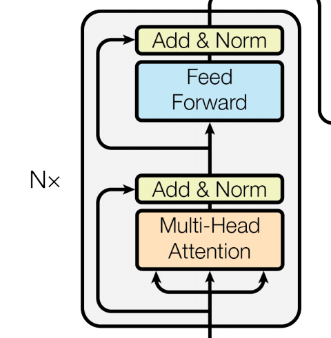 [Image source: Vaswani et al. (2017)]
Now we can pass on the input to the encoder. There are two modules related to the encoder - nn.TransformerEncoderLayer and nn.TransformerEncoder. Remember that the encoder is a stack of $N$ identical layers ($N = 6$ in the Vaswani et al. paper). Each “layer” consists of multi-head attention and position-wise feed-forward networks.
nn.TransformerEncoderLayer generates a single layer and nn.TransformerEncoder basically stacks up $N$ copies of that instance. The output shapes from all layers are identical, making this much simple. Also note that we can specify the dropout rate with the dropout parameter, making nodes in each layer “dropped out” to prevent overfitting.
enc_layer = nn.TransformerEncoderLayer(EMBEDDING_DIM, NUM_HEADS, HIDDEN_SIZE, DROPOUT)
memory = enc_layer(src)
print(memory.shape)                      # (SEQ_LEN, BATCH_SIZE, EMBEDDING_DIM)
nn.TransformerEncoder stacks up NUM_LAYERS copies of encoder layers. The outputs from the encoder are named “memory,” indicating that the encoder memorizes information from source sequences and passes them on to the decoder.
encoder = nn.TransformerEncoder(enc_layer, num_layers = NUM_LAYERS)
memory = encoder(src)
print(memory.shape)                     # (SEQ_LEN, BATCH_SIZE, EMBEDDING_DIM)
Decoder
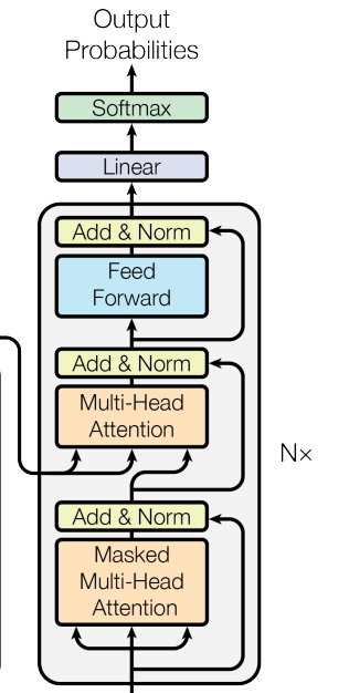 [Image source: Vaswani et al. (2017)]
The decoder architecture is similar, but it has two multi-head attention networks to (1) process the “memory” from the encoder and (2) extract information from target sequences. Therefore, nn.TransformerDecoderLayer and nn.TransformerDecoder have two inputs, tgt and memory.
dec_layer = nn.TransformerDecoderLayer(EMBEDDING_DIM, NUM_HEADS, HIDDEN_SIZE, DROPOUT)
decoder = nn.TransformerDecoder(dec_layer, num_layers = NUM_LAYERS)
transformer_output = decoder(tgt, memory)
print(transformer_output.shape)        # (SEQ_LEN, BATCH_SIZE, EMBEDDING_DIM)
Final dense layer
To classify each token, we need to have an additional layer to calculate the probabilities. The output size of the final dense layer is equivalent to the vocabulary size of target language.
dense = nn.Linear(EMBEDDING_DIM, DEU_VOCAB_SIZE)
final_output = dense(transformer_output)
print(final_output.shape)             # (SEQ_LEN, BATCH_SIZE, EMBEDDING_DIM)
Putting it together
Now, we can just put all things together and create a blueprint for the Transformer network that can be used for most of sequence-to-sequence mapping tasks.
class TransformerNet(nn.Module):
  def __init__(self, num_src_vocab, num_tgt_vocab, embedding_dim, hidden_size, nheads, n_layers, max_src_len, max_tgt_len, dropout):
    super(TransformerNet, self).__init__()
    # embedding layers
    self.enc_embedding = nn.Embedding(num_src_vocab, embedding_dim)
    self.dec_embedding = nn.Embedding(num_tgt_vocab, embedding_dim)

    # positional encoding layers
    self.enc_pe = PositionalEncoding(embedding_dim, max_len = max_src_len)
    self.dec_pe = PositionalEncoding(embedding_dim, max_len = max_tgt_len)

    # encoder/decoder layers
    enc_layer = nn.TransformerEncoderLayer(embedding_dim, nheads, hidden_size, dropout)
    dec_layer = nn.TransformerDecoderLayer(embedding_dim, nheads, hidden_size, dropout)
    self.encoder = nn.TransformerEncoder(enc_layer, num_layers = n_layers)
    self.decoder = nn.TransformerDecoder(dec_layer, num_layers = n_layers)

    # final dense layer
    self.dense = nn.Linear(embedding_dim, num_tgt_vocab)
    self.log_softmax = nn.LogSoftmax()

  def forward(self, src, tgt):
    src, tgt = self.enc_embedding(src).permute(1, 0, 2), self.dec_embedding(tgt).permute(1, 0, 2)
    src, tgt = self.enc_pe(src), self.dec_pe(tgt)
    memory = self.encoder(src)
    transformer_out = self.decoder(tgt, memory)
    final_out = self.dense(transformer_out)
    return self.log_softmax(final_out)
model = TransformerNet(ENG_VOCAB_SIZE, DEU_VOCAB_SIZE, EMBEDDING_DIM, HIDDEN_SIZE, NUM_HEADS, NUM_LAYERS, MAX_SENT_LEN, MAX_SENT_LEN, DROPOUT).to(DEVICE)
criterion = nn.NLLLoss()
optimizer = torch.optim.Adam(model.parameters(), lr = LEARNING_RATE)
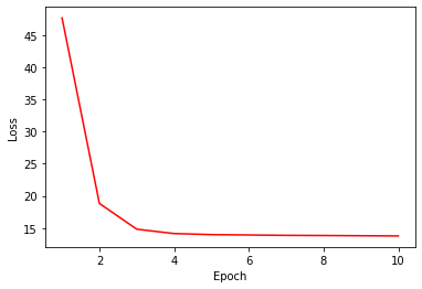
After training, you can see that this Transformer network shows more stable and robust result compared to the one we trained in the previous posting.
%%time
loss_trace = []
for epoch in tqdm(range(NUM_EPOCHS)):
  current_loss = 0
  for i, (x, y) in enumerate(train_loader):
    x, y  = x.to(DEVICE), y.to(DEVICE)
    outputs = model(x, y)
    loss = criterion(outputs.permute(1, 2, 0), y)
    optimizer.zero_grad()
    loss.backward()
    optimizer.step()
    current_loss += loss.item()
  loss_trace.append(current_loss)

# loss curve
plt.plot(range(1, NUM_EPOCHS+1), loss_trace, 'r-')
plt.xlabel('Epoch')
plt.ylabel('Loss')
plt.show()