
케라스와 함께하는 쉬운 딥러닝 (10) - CNN 모델 개선하기 1
04 May 2018 | Python Keras Deep Learning 케라스합성곱 신경망 4 - CNN 모델 개선하기 1
Objective: 케라스로 개선된 CNN 모델을 만들어 본다.
지난 포스팅에서 케라스로 간단한 CNN 모델을 만들고 이를 Digits 데이터 셋에 적용해보았다.
이번 포스팅에서는 지난 포스팅의 간단한 CNN 모델에서 나아가, 이를 더 깊게(deep cnn) 만들어 보자.
깊어지는 합성곱 신경망(Deep CNN)
2012년 AlexNet이 제안되기 이전의 뉴럴 네트워크는 대부분 레이어가 몇 개 없는 얕은 구조(shallow structure)를 가지고 있었다. 하지만 AlexNet이 ILSVRC 2012에서 8개의 레이어로 깊은 구조가 복잡한 데이터를 학습하는 데 효과적이라는 것을 증명한 이후로 CNN은 갈수록 깊어져 2015년 ILSVRC의 우승자인 ResNet은 152개의 레이어를 자랑한다.
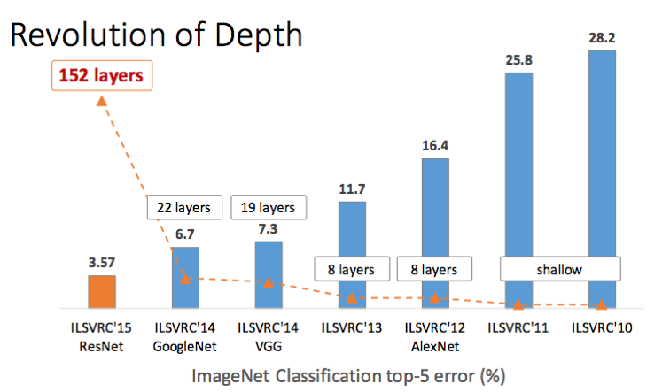
깊어진 CNN은 더욱 많은 feature extraction 연산과 비선형 활성 함수(nonlinear activation function)를 통해 이미지와 같은 복잡한 데이터의 추상적인 표현(abstract representation)을 캐치해낼 수 있다는 강점을 가지지만, 한편으로는 파라미터의 숫자가 많아지면서 경사하강법을 통한 학습과정이 까다로워지고, 과적합(overfitting)의 문제가 발생하기도 한다.
그러므로, 깊어진 CNN은 모델의 학습과 검증에 있어 대부분의 복잡한 뉴럴 네트워크가 그렇듯, 더욱 주의를 요한다.
MNIST 데이터 셋 불러오기
MLP에서도 사용했던 MNIST 데이터 셋을 불러온다. 그때와 다른 점이 있다면, 그때는 MLP 모델에 입력하기 위해 (28, 28, 1) 짜리 사이즈의 데이터를 flatten해 784차원의 1차원 벡터로 만들었다면, 여기에서는 3차원 이미지 데이터를 그대로 사용한다는 것이다.
import numpy as np
import matplotlib.pyplot as plt

from keras.datasets import mnist
from keras.utils.np_utils import to_categorical

(X_train, y_train), (X_test, y_test) = mnist.load_data()
# reshaping X data: (n, 28, 28) => (n, 28, 28, 1)
X_train = X_train.reshape((X_train.shape[0], X_train.shape[1], X_train.shape[2], 1))
X_test = X_test.reshape((X_test.shape[0], X_test.shape[1], X_test.shape[2], 1))
# converting y data into categorical (one-hot encoding)
y_train = to_categorical(y_train)
y_test = to_categorical(y_test)

print(X_train.shape, X_test.shape, y_train.shape, y_test.shape)
(60000, 28, 28, 1), (10000, 28, 28, 1), (60000, 10), (10000, 10)
간단한 CNN 모델 만들기
지난 포스팅에서 만들었던 것과 비슷하게, 하나의 convolution 레이어와 pooling 레이어를 가진 CNN 모델을 만들어 보자.
from keras.models import Sequential
from keras import optimizers
from keras.layers import Dense, Activation, Flatten, Conv2D, MaxPooling2D

def basic_cnn():
    model = Sequential()

    model.add(Conv2D(input_shape = (X_train.shape[1], X_train.shape[2], X_train.shape[3]), filters = 50, kernel_size = (3,3), strides = (1,1), padding = 'same'))
    model.add(Activation('relu'))
    model.add(MaxPooling2D(pool_size = (2,2)))

    # prior layer should be flattend to be connected to dense layers
    model.add(Flatten())
    # dense layer with 50 neurons
    model.add(Dense(50, activation = 'relu'))
    # final layer with 10 neurons to classify the instances
    model.add(Dense(10, activation = 'softmax'))

    adam = optimizers.Adam(lr = 0.001)
    model.compile(loss = 'categorical_crossentropy', optimizer = adam, metrics = ['accuracy'])

    return model

model = basic_cnn()
model.summary()
model.summary() 를 통해 모델의 대략적인 구조를 파악해볼 수 있다. 간단한 CNN 모델은 491,060개의 학습 가능한 파라미터를 가진다.
Layer (type)                 Output Shape              Param #
=================================================================
conv2d_13 (Conv2D)           (None, 28, 28, 50)        500
_________________________________________________________________
activation_4124 (Activation) (None, 28, 28, 50)        0
_________________________________________________________________
max_pooling2d_8 (MaxPooling2 (None, 14, 14, 50)        0
_________________________________________________________________
flatten_6 (Flatten)          (None, 9800)              0
_________________________________________________________________
dense_11 (Dense)             (None, 50)                490050
_________________________________________________________________
dense_12 (Dense)             (None, 10)                510
=================================================================
Total params: 491,060
Trainable params: 491,060
Non-trainable params: 0
_________________________________________________________________
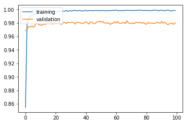
모델을 학습시키고 학습 과정을 시각화해 본다.
history = model.fit(X_train, y_train, batch_size = 50, validation_split = 0.2, epochs = 100, verbose = 0)

plt.plot(history.history['acc'])
plt.plot(history.history['val_acc'])
plt.legend(['training', 'validation'], loc = 'upper left')
plt.show()
학습 결과를 검증해 본다.
results = model.evaluate(X_test, y_test)
print('Test accuracy: ', results[1])
Test accuracy: 0.9811
학습 및 검증 결과 검증 정확도 98.11%로 간단한 모델 치고는 나쁘지 않은 성능이 나왔다. 이번에는 이를 조금 더 깊게 만들어 정확도를 더 끌어올릴 수 있는지 확인해 보자.
깊은 CNN 모델 만들기
6개의 convolution 레이어와 3개의 pooling 레이어를 가진 깊은 cnn 구조를 생성해 보자.
def deep_cnn():
    model = Sequential()

    model.add(Conv2D(input_shape = (X_train.shape[1], X_train.shape[2], X_train.shape[3]), filters = 50, kernel_size = (3,3), strides = (1,1), padding = 'same'))
    model.add(Activation('relu'))
    model.add(Conv2D(filters = 50, kernel_size = (3,3), strides = (1,1), padding = 'same'))
    model.add(Activation('relu'))
    model.add(MaxPooling2D(pool_size = (2,2)))
    model.add(Conv2D(filters = 50, kernel_size = (3,3), strides = (1,1), padding = 'same'))
    model.add(Activation('relu'))
    model.add(Conv2D(filters = 50, kernel_size = (3,3), strides = (1,1), padding = 'same'))
    model.add(Activation('relu'))
    model.add(MaxPooling2D(pool_size = (2,2)))
    model.add(Conv2D(filters = 50, kernel_size = (3,3), strides = (1,1), padding = 'same'))
    model.add(Activation('relu'))
    model.add(Conv2D(filters = 50, kernel_size = (3,3), strides = (1,1), padding = 'same'))
    model.add(Activation('relu'))
    model.add(MaxPooling2D(pool_size = (2,2)))

    # prior layer should be flattend to be connected to dense layers
    model.add(Flatten())
    # dense layer with 50 neurons
    model.add(Dense(50, activation = 'relu'))
    # final layer with 10 neurons to classify the instances
    model.add(Dense(10, activation = 'softmax'))

    adam = optimizers.Adam(lr = 0.001)
    model.compile(loss = 'categorical_crossentropy', optimizer = adam, metrics = ['accuracy'])

    return model

model = deep_cnn()
model.summary()
아래 summary에서 보듯이 학습 가능한 파라미터의 수가 136,310개로 간단한 cnn 모델에 비해 훨씬 많은 것을 확인해볼 수 있다.
_________________________________________________________________
Layer (type)                 Output Shape              Param #
=================================================================
conv2d_22 (Conv2D)           (None, 28, 28, 50)        500
_________________________________________________________________
activation_4133 (Activation) (None, 28, 28, 50)        0
_________________________________________________________________
conv2d_23 (Conv2D)           (None, 28, 28, 50)        22550
_________________________________________________________________
activation_4134 (Activation) (None, 28, 28, 50)        0
_________________________________________________________________
max_pooling2d_13 (MaxPooling (None, 14, 14, 50)        0
_________________________________________________________________
conv2d_24 (Conv2D)           (None, 14, 14, 50)        22550
_________________________________________________________________
activation_4135 (Activation) (None, 14, 14, 50)        0
_________________________________________________________________
conv2d_25 (Conv2D)           (None, 14, 14, 50)        22550
_________________________________________________________________
activation_4136 (Activation) (None, 14, 14, 50)        0
_________________________________________________________________
max_pooling2d_14 (MaxPooling (None, 7, 7, 50)          0
_________________________________________________________________
conv2d_26 (Conv2D)           (None, 7, 7, 50)          22550
_________________________________________________________________
activation_4137 (Activation) (None, 7, 7, 50)          0
_________________________________________________________________
conv2d_27 (Conv2D)           (None, 7, 7, 50)          22550
_________________________________________________________________
activation_4138 (Activation) (None, 7, 7, 50)          0
_________________________________________________________________
max_pooling2d_15 (MaxPooling (None, 3, 3, 50)          0
_________________________________________________________________
flatten_9 (Flatten)          (None, 450)               0
_________________________________________________________________
dense_17 (Dense)             (None, 50)                22550
_________________________________________________________________
dense_18 (Dense)             (None, 10)                510
=================================================================
Total params: 136,310
Trainable params: 136,310
Non-trainable params: 0
_________________________________________________________________
history = model.fit(X_train, y_train, batch_size = 50, validation_split = 0.2, epochs = 100, verbose = 0)

plt.plot(history.history['acc'])
plt.plot(history.history['val_acc'])
plt.legend(['training', 'validation'], loc = 'upper left')
plt.show()
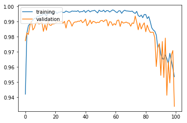
모델의 정확도가 계속 들쭉날쭉하며, 특히 80 에포크 후에 모델의 정확도가 전반적으로 떨어지는 것을 볼 수 있다.
results = model.evaluate(X_test, y_test)
print('Test accuracy: ', results[1])
Test accuracy: 0.9368
최종 검증 정확도도 93.68%로 깊은 모델을 만들었음에도 불구하고 간단한 모델에 비해서 6%가량 낮은 정확도를 보이는 것을 볼 수 있다. 서두에서 깊은 모델의 경우 학습이 어렵다고 말한 문제를 반영하는 것으로 추측해볼 수 있다.
이제 다음 포스팅에서 깊은 모델을 어떻게 더 잘 학습시킬 수 있는지에 대해 알아보자.
전체 코드
본 실습의 전체 코드는 여기에서 열람하실 수 있습니다!