So far, we have covered memory-based collaborative filtering (CF) methods and experimented with the k-Nearest Neighbors (k-NN) algorithm in Python. From now on, let’s switch gears and dig into model-based CF methods.

Model-based CF

We have seen that memory-based CF methods infer ratings based on the memory of previous user-item interaction records. Model-based CF methods are similar in that they make guesses based on previous interaction records. However, instead of relying on pre-computed similarity (or distance) measures, model-based methods employ various prediction models to capture the latent relationship between users and items.

Baseline predictor

In fact, we have already implemented a very simple algorithm for model-based CF, which is the baseline predictor. In general, most recommendation problems show inherent biases, which are overall tendencies that can be generalized on a dataset-level. For instance, some users are generous that they give better ratings than others on average. At the same time, some items have inherently more appealing features than others, resulting in better ratings on average. If you look at the top-100 movies in IMDb, they are rated higher than other movies among the vast majority of users.

Therefore, the baseline estimator tries to guess the magnitude of individual user and item biases. The equation for the estimator is:

\begin{equation} b_{ui} = \mu + b_u + b_i , \end{equation}

where $\mu$ is the average rating across all user-item interactions and $b_u$ and $b_i$ refer to biases for user $u$ and item $i$, respectively. Hence, the baseline predictor tries to quantify how the user and item of interest deviate from the overall average. This is a simple, yet very powerful, idea. In the previous posting, we have seen that it is difficult to beat the baseline predictor with k-NN without incorporating it.

Latent factor models

However, the baseline model has apparent limitations. To start with, it doesn’t consider individual preferences and granular heterogeneity in item features. For instance, Krusty might be a generous and easy-going reviewer in general, but he could be very critical about comedy movies (since he is a clown). Also, Tony could give harsh ratings to most of the movies, but he might have predilections for De Niro movies such as Goodfellas and Irishman (since he is a mafia). Nonetheless, the baseline model aggregates all those information on user- and item-levels, forgoing the granularity.

Therefore, more sophisticated models, namely latent factor models, have been proposed to model complex collaborative patterns. Such patterns are highly non-linear and non-transitive. One of the seminal models have been popularized during the Netflix Prize (Funk 2006), the matrix factorization (MF) model. Recall that memory-based models are good at memorization in general, whereas model-based methods are good at generalization. MF-based models are suited for such generalization tasks.

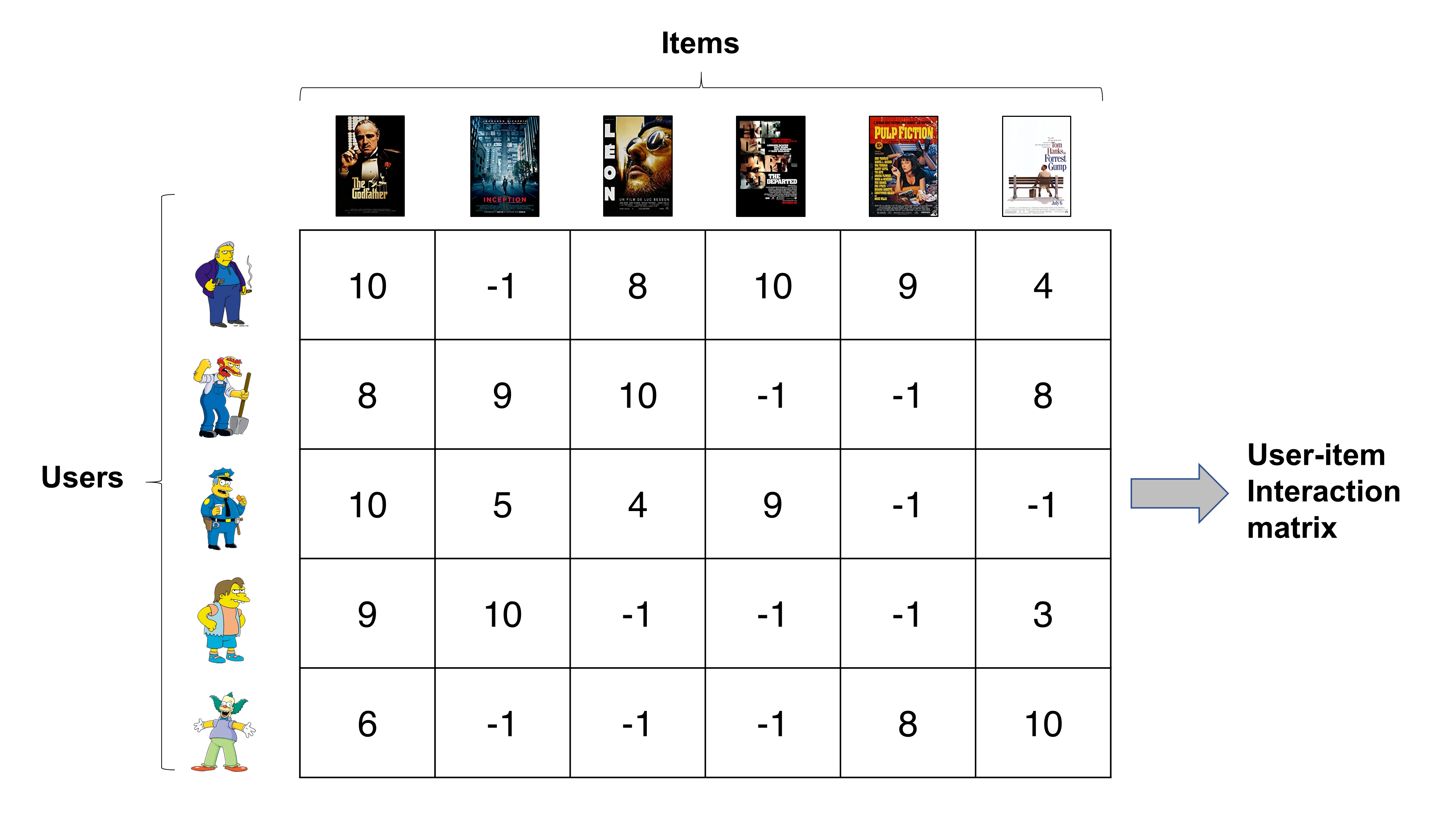
Do you remember the user-item interaction matrix comprising rating records? MF models attempt to decompose that matrix into two matrices that characterize users and items, respectively. In doing so, the difference between the predicted ratings and actual ratigns are minimized. We will look into MF in detail in the following postings.

[Image source]

Deep recommender systems

MF is a great model with apparent strengths. However, it also has some limitations as recommendation problems gets more complicated. Sometimes, the model architeture is too simple to capture highly complex interaction patterns. Also, it cannot incorporate side information reflecting the context and content. With recent advances in big data, more and more recommendation problems require the prediction model to ingest diverse modes of data such as image and text for optimal performance. Hence, more and more systems adopt deep learning architecture for prediction.

Deep learning provides a great amount of flexibility in terms of model architecture and input data, e.g., neural collaborative filtering (He et al. 2017) and wide & deep learning (Cheng et al. 2016). In the following postings, we will also look at recent developments in deep recommender systems.

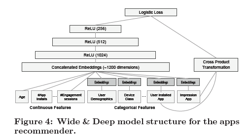[Image source: Cheng et al. (2016)]

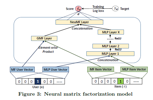[Image source: He et al. (2017)]

References

• Cheng, H. T., Koc, L., Harmsen, J., Shaked, T., Chandra, T., Aradhye, H., … & Anil, R. (2016, September). Wide & deep learning for recommender systems. In Proceedings of the 1st workshop on deep learning for recommender systems (pp. 7-10).
• Funk, S. (2006) Netflix Update: Try This at Home. (https://sifter.org/~simon/journal/20061211.html)
• He, X., Liao, L., Zhang, H., Nie, L., Hu, X., & Chua, T. S. (2017, April). Neural collaborative filtering. In Proceedings of the 26th international conference on world wide web (pp. 173-182).
• Matrix Factorization (https://developers.google.com/machine-learning/recommendation/collaborative/matrix)
• Koren, Y. (2010). Factor in the neighbors: Scalable and accurate collaborative filtering. ACM Transactions on Knowledge Discovery from Data (TKDD), 4(1), 1-24.
• Ricci, F., Rokach, L., & Shapira, B. (2011). Introduction to recommender systems handbook. In Recommender systems handbook (pp. 1-35). Springer, Boston, MA.