
Attention in Neural Networks - 6. Sequence-to-Sequence (Seq2Seq) (5)
07 Feb 2020 | Attention mechanism Deep learning PytorchAttention Mechanism in Neural Networks - 6. Sequence-to-Sequence (Seq2Seq) (5)
In the previous posting, we trained and evaluated the RNN Encoder-Decoder model by Cho et al. (2014) with Pytorch. In this posting, let’s look into another very similar, yet subtly different, Seq2Seq model proposed by Sutskever et al. (2014)
Model
As mentioned, the model by Sutskever et al. (2014) is largely similar to the one proposed by Cho et al. (2014). However, there are some subtle differences that can make the model more powerful. The key differences outlined in the paper are
- Deep LSTM layers: Sutskever et al. (2014) claim that using deep LSTMs can significantly outperform shallow LSTMs which have only a single layer. Therefore, they use LSTMs with four layers and empirically show that doing so results in better performances.
- Reversing the order of input sequences: By reversing the order of the input sequence, they claim that inputs and outputs are more aligned in a sense. For instance, assume mapping a sequence a, b, c to $\alpha, \beta, \gamma$. By reordering the source sequence by c, b, a, a is closer to $\alpha$, b is closer to $\beta$. By doing so, it is easier for the algorihtm to “establish communication” between the source and target.
Import packages & download dataset
First things first, we need to import necessary packages and download the datset. This is same as the previous postings, so you can skip and go on to the next section if you are already familiar with.
import re
import torch
import numpy as np
import torch.nn as nn
from matplotlib import pyplot as plt
from tqdm import tqdm

!wget https://www.manythings.org/anki/deu-eng.zip
!unzip deu-eng.zip

with open("deu.txt") as f:
  sentences = f.readlines()

# number of sentences
len(sentences)
204574
Data processing
In processing the data, there is only one difference. We need to change the order of the source sequence. This can be easily accomplished by reversing each list in the input sentence.
First, we start with cleaning and tokenizing the text data.
NUM_INSTANCES = 50000
eng_sentences, deu_sentences = [], []
eng_words, deu_words = set(), set()
for i in tqdm(range(NUM_INSTANCES)):
  rand_idx = np.random.randint(len(sentences))
  # find only letters in sentences
  eng_sent, deu_sent = ["<sos>"], ["<sos>"]
  eng_sent += re.findall(r"\w+", sentences[rand_idx].split("\t")[0])
  deu_sent += re.findall(r"\w+", sentences[rand_idx].split("\t")[1])

  # change to lowercase
  eng_sent = [x.lower() for x in eng_sent]
  deu_sent = [x.lower() for x in deu_sent]
  eng_sent.append("<eos>")
  deu_sent.append("<eos>")

  # add parsed sentences
  eng_sentences.append(eng_sent)
  deu_sentences.append(deu_sent)

  # update unique words
  eng_words.update(eng_sent)
  deu_words.update(deu_sent)

eng_words, deu_words = list(eng_words), list(deu_words)
This is where we have to pay attention. We can reverse each source sequence with the reverse() function. This can be done after or before converting them into array of indices.
# encode each token into index
for i in tqdm(range(len(eng_sentences))):
  temp = [eng_words.index(x) for x in eng_sentences[i]]
  temp.reverse()
  eng_sentences[i] = temp
  deu_sentences[i] = [deu_words.index(x) for x in deu_sentences[i]]
Setting parameters
Parameters are also set to in a similar fashion. Nonetheless, we have to add additional parameter, which determines the number of layers in LSTM. In the paper, they propose four-layer LSTM and we follow it. However, you can surely tune this according to the size of the dataset and computing resource you have.
MAX_SENT_LEN = len(max(eng_sentences, key = len))
ENG_VOCAB_SIZE = len(eng_words)
DEU_VOCAB_SIZE = len(deu_words)
NUM_EPOCHS = 10
HIDDEN_SIZE = 128
EMBEDDING_DIM = 30
NUM_LAYERS = 4
DEVICE = torch.device('cuda')
Encoder and Decoder
The encoder and decoder are also similarly defined, having additional parameter of num_layers, which indicates the number of layers in each LSTM.
class Encoder(nn.Module):
  def __init__(self, vocab_size, hidden_size, embedding_dim, num_layers):
    super(Encoder, self).__init__()
    self.hidden_size = hidden_size
    self.num_layers = num_layers

    self.embedding = nn.Embedding(vocab_size, embedding_dim)
    self.lstm = nn.LSTM(embedding_dim, hidden_size, num_layers)

  def forward(self, x, h0, c0):
    x = self.embedding(x).view(1, 1, -1)
    out, (h0, c0) = self.lstm(x, (h0, c0))
    return out, (h0, c0)

class Decoder(nn.Module):
  def __init__(self, vocab_size, hidden_size, embedding_dim, num_layers):
    super(Decoder, self).__init__()
    self.hidden_size = hidden_size
    self.num_layers = num_layers

    self.embedding = nn.Embedding(vocab_size, embedding_dim)
    self.lstm = nn.LSTM(embedding_dim, hidden_size, num_layers)
    self.dense = nn.Linear(hidden_size, vocab_size)
    self.softmax = nn.LogSoftmax(dim = 1)

  def forward(self, x, h0, c0):
    x = self.embedding(x).view(1, 1, -1)
    x, (h0, c0) = self.lstm(x, (h0, c0))
    x = self.softmax(self.dense(x.squeeze(0)))
    return x, (h0, c0)
encoder = Encoder(ENG_VOCAB_SIZE, HIDDEN_SIZE, EMBEDDING_DIM, NUM_LAYERS).to(DEVICE)
decoder = Decoder(DEU_VOCAB_SIZE, HIDDEN_SIZE, EMBEDDING_DIM, NUM_LAYERS).to(DEVICE)
Training
In the training phase, what gets different is the size of the hidden state (h0) and the cell state (c0). In the previous posting we could set them as (1, 1, HIDDEN_SIZE) since we had only one layer and one direction. However, it has to be changed to (NUM_LAYERS, 1, HIDDEN_SIZE) since we have multiple layers. In general, the size of hidden and cell states for RNN is (NUM_LAYERS * NUM_DIRECTION, BATCH_SIZE, HIDDEN_SIZE). We will come back to this again later when we are dealing with bidirectional RNNs.
%%time
encoder_opt = torch.optim.Adam(encoder.parameters(), lr = 0.01)
decoder_opt = torch.optim.Adam(decoder.parameters(), lr = 0.01)
criterion = nn.NLLLoss()
current_loss = []

for i in tqdm(range(NUM_EPOCHS)):
  for j in tqdm(range(len(eng_sentences))):
    source, target = eng_sentences[j], deu_sentences[j]
    source = torch.tensor(source, dtype = torch.long).view(-1, 1).to(DEVICE)
    target = torch.tensor(target, dtype = torch.long).view(-1, 1).to(DEVICE)

    loss = 0
    h0 = torch.zeros(encoder.num_layers, 1, encoder.hidden_size).to(DEVICE)
    c0 = torch.zeros(encoder.num_layers, 1, encoder.hidden_size).to(DEVICE)

    encoder_opt.zero_grad()
    decoder_opt.zero_grad()

    enc_output = torch.zeros(MAX_SENT_LEN, encoder.hidden_size)
    for k in range(source.size(0)):
      out, (h0, c0) = encoder(source[k].unsqueeze(0), h0, c0)
      enc_output[k] = out.squeeze()

    dec_input = torch.tensor([[deu_words.index("<sos>")]]).to(DEVICE)
    for k in range(target.size(0)):
      out, (h0, c0) = decoder(dec_input, h0, c0)
      _, max_idx = out.topk(1)
      dec_input = max_idx.squeeze().detach()
      loss += criterion(out, target[k])
      if dec_input.item() == deu_words.index("<eos>"):
        break

    loss.backward()
    encoder_opt.step()
    decoder_opt.step()
  current_loss.append(loss.item())
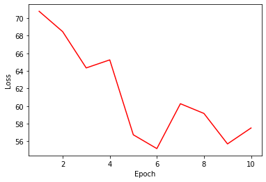
Let’s try plotting the loss curve. It can be observed that the loss drops abruptly around the fifth epoch.
# loss curve
plt.plot(range(1, NUM_EPOCHS+1), current_loss, 'r-')
plt.xlabel('Epoch')
plt.ylabel('Loss')
plt.show()
References
- NLP FROM SCRATCH: TRANSLATION WITH A SEQUENCE TO SEQUENCE NETWORK AND ATTENTION
- Sutskever et al. (2014)
In this posting, we looked into implementing the Seq2Seq model by Sutskever et al. (2014). In the following postings, let’s look into the details of the Seq2Seq model with the natural extension of alignment networks.