Attention Mechanism in Neural Networks - 17. Transformer (1)

In the previous posting, we implemented the hierarchical attention network architecture with Pytorch. Now let’s move on and take a look into the Transformer. During the last few years, the Transformer has truly revolutionized the NLP and deep learning field. As mentioned in the deep learning state-of-the-art 2020 posting, the Bidirectional Encoder Representations from Transformers (BERT) achieved cutting-edge results in many major NLP tasks such as sentence classification and question answering. Furthermore, a number of BERT-based models demonstrating superhuman performances, such as XLNET, RoBERTa, DistilBERT, and ALBERT have been proposed recently.

The Transformer neural network architecture, proposed by Vaswani et al. (2017) is relatively simple and quick to train compared to deep RNNs or CNNs. However, some alien terminologies, e.g., multi-head attention and positional encoding, make it daunting for beginners. In this posting, let’s take a first step for a beginner-friendly look at the architecture.

Query, keys, values

In the abstract, what attention does is calculating the weights for each element in values ($V$), given queries ($Q$) and keys ($K$). Therefore, it can be said that the relationship between $Q$ and $K$ determines the weights. In the RNN Encoder-Decoder model that we have seen so far, the keys and values are identical, which are the hidden states from the encoder.

\begin{equation} K = V = (h_1, h_2, … h_n) \end{equation}

Wheareas $Q$ is the (current) hidden state of the decoder, i.e., $s_i$. The weights for $V$ are computed by the alignment model ($a$) that aligns $Q$ and $K$. The normalized weights ($\alpha_{ik}$) are then used to compute the context vector ($c_t$). As we have seen in the previous posting, there are many choices for the alignment model, i.e., how to compute $c_t$.

Scaled dot-product attention

As mentioned, there are many possible choices for scoring the weights for $V$, such as general, concat, and dot product. For details, you can refer to Luong et al. (2015)

The scoring function recommended by Vaswani et al. (2017) is the scaled dot-product function, which is a slight variant of the dot function, which basically applies dot product on the $Q$ and $K$, or $h$ and $s$. The scaled-dot function scales the dot product between $Q$ and $K$ with square-root of the dimensionality of $V$, i.e., $\sqrt{d_k}$. Therefore,

\begin{equation} Attention(Q, K, V) = softmax(\frac{QK^{T}}{\sqrt{d_k}})V \end{equation}

The reason for scaling is to prevent the cases where gradients gets extremely small by dot products growing too large.

We suspect that for large values of $d_k$, the dot products grow large in magnitude, pushing the softmax function into regions where it has extremely small gradients (Vaswani et al. 2017, pp. 4)

Self-attention

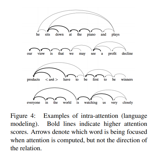
One of the key characteristics of the Transformer that differentiates from RNN Encoder-Decoder and its variants is the utilization of self-attention. Self-attention, or intra-attention, attempts to discover patterns among inputs in a single sequence, rather than input/output pairs from two sequences. This process, initially utilized by the Long Short-Term Memory Networks (Cheng et al. 2016), resembles the human reading process.

[Image source: Cheng et al. (2016)]

Since there is only one sequence to model, the query, key, and value are the same in self-attention networks ($Q = K = V$). Also, since there is no RNN cells in the network, they are not hidden states. Rather, they are positional-encoded embedded sequence inputs. We will see what positional encoding is in the following section, so don’t worry.

The self-attention mechanism is extremely powerful that the Transformer completely eschews traditional choices for sequence modeling, i.e., RNNs and CNNs. And this was such a revolutionary proposal that the authors dedicated an entire section (specifically, Section 4) advocating the use of self-attention. Below are three reasons that the authors opted for self-attention with feedforward layers.

One is the total computational complexity per layer. Another is the amount of computation that can be parallelized, as measured by the minimum number of sequential operations required. The third is the path length between long-range dependencies in the network (Vaswani et al. 2017, pp. 6)

Positional encoding

As the Transformer eschews CNN and RNN, additional information regarding the order of the sequence should be injected.

Since our model contains no recurrence and no convolution, in order for the model to make use of the order of the sequence, we must inject some information about the relative or absolute position of the tokens in the sequence. To this end, we add “positional encodings” to the input embeddings at the bottoms of the encoder and decoder stacks (Vaswani et al. 2017, pp. 5-6)

Among many choices for positional encoding, the authors used sine and cosine functions. For each position $pos$ in the sequence and dimension $i$, encodings are obtained with below functions.

The dimension ($i$) spans through 1 to $d_{model}$, which is the dimensionality of the embedding space. Therefore, outputs from positional encoding have the same tensor size as the embedded sequences. They are added up and passed onto the next layer, which is multi-head attention.

Multi-head attention

Multi-head attention is basically concatenating multiple attention results and projecting it with linear transformation ($W^O$).

\begin{equation} MultiHead(Q, K, V) = Concat(head_1, head_2, …, head_h)W^O \end{equation}

To minimize the compuational cost, the query, key and value are projected to lower-dimensional space ($d_k, d_k, d_v$) with linear transformations ($W_i^Q, W_i^K, W_i^V$). It is claimed that the total computational cost is kept similar to that of single attention with full dimensionality.

\begin{equation} head_i = Attention(QW_i^Q, KW_i^K, VW_i^V) \end{equation}

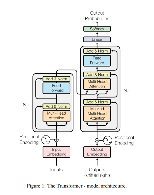
Finally, we have gone through all of the key building blocks of Transformer. Now you would be in a better position to understand the architecture of Transformer outlined in below figure by Vaswani et al. (2017). It is not required to entirely understand the mathematics and details of each mechanism (at least I can’t, to be honest), but good to have a general idea of how the network works.

[Image source: Vaswani et al. (2017)]

In the next posting, let’s try implementing the Transformer with Pytorch. Good new is that Pytorch provides nn.Transformer and related modules that makes implemenation extremely easy. See you in the next posting!

References

• Vaswani et al. (2017)
• Cheng et al. 2016