Recommender systems lie at the heart of modern information systems we are using on a daily basis. It is difficult to imagine many services without the recommendation functionalities. For example, Amazon without product suggestion and Netflix without video recommendation service would be virtually good-for-nothing. It has been reported that about 80% of streaming choices in Netflix is influenced by recommendations, wheareas sarching accounts for mere 20% (Gomez-Uribe and Hunt 2015).

The real value produced by an information provider comes in locating, filtering, and communicating what is useful to the customer. (Varian and Shapiro 1998)

With that said, in this posting series, let’s delve into recommender systems and how to implement them with Python. Recommender systems, especially those are deployed in the wild are very complex and require a huge amount of feature engineering and modeling. But in this posting series, we will minimize such effort by effectively utilizing Python packages such as fast.ai and Surprise. I will specifically focusing on collaborative filtering methods, in which a great amount of progress was made during the last decade. Don’t know what collaborative filtering is? Don’t worry, you will get to know it just after you read this posting!

Types of recommender systems

Although there is a fine line between them, there are largely three types of recommender systems. They are (1) content-based, (2) collaborative filtering **, and **(3) hybrid recommender systems. Let’s have a brief look at each of them and what are their pros and cons.

Content-based recommender systems

Content-based systems try to recommend items that are similar to the items that the user likes. For instance, if a Netflix user likes the movie Iron Man, we can recommend the movie Avengers to the user since Iron Man and Avengers are likely to have high content similarity. Alternatively, we can find a set of similar users and see which items those users like, among items that the user of interest had not liked yet.

For instance, Amazon’s “products related to this item” recommendations are likely to be suggested by picking items that are similar to the product that the user is viewing.

As many could have noticed, measuring the similarity between items is a fundamental task in designing virtually any content-based recommender system. In practice, there are a wide array of methods used to measure it, ranging from basic item features and meta information to text analysis and graphs. And this is where anyone can be creative since there should be tons of ways to define the similarity function.

[Image Source](https://en.wikipedia.org/wiki/The_Product_Space)

However, defining such similarity function might be tricky and burdensome since many items do not have explicit features that can be easily quantified. Besides, it can require a great amount of compuational resources to calculate pairwise similarity scores, especially when the number of products is large. Fortunately, some of those limitations can be tackled with the collaborative filtering approach, which will be explained in the following subsection.

Collaborative filtering recommender systems

The collaborative filtering approach has two major steps - (1) identify users having similar likings in the past and (2) suggest items that those users liked the most. In the first step, we have to find users that have similar liking patterns with the user of interest. Then, we rank the items in the recommendation pool based on those users’ preferences. Thus, collaborative filtering is referred to as “people-to-people” correlation.

Going back to the movie recommendations example, let us assume that there are three users A, B, and C, and we want to recommend a new movie to user C. You can see that the preferences of users A and C are highly similar - they both liked the movies Batman Begins and Midnight in Paris. And since A also liked the movie Joker and C didn’t, we can confidently recommend the movie to C. The reality is much more complicated that this, but you will get the idea.

As mentioned, collaborative filtering is where a great amount of research has been carried out recently. Besides, collaborative filtering methods are widely used in practice to recommend various products to users. One of the reasons is that with advancements in information technology, we now have the tools to store, process, and analyze large-scale interaction patterns between users and items. This was not possible before tech giants such as FAANG started to recognize the value of such data and utilize them for recommendation.

[Image Source: Gomez-Uribe and Hunt 2015]

Nevertheless, collaborative filtering systems are far from perfect. The most critical one arises from the classical cold-start problem, in which we do not have any past record of a user. In such case, it is difficult to find users that have similar preferences and to recommend items, accordingly. Assume that a new user (D) creates an account to a streaming service. We do not have information, so it is hard to make a recommendation for D. And this is why Netflix asks for the shows that you liked when you first make your account - to avoid the cold start problem and start recommendation right away, which accounts for 80% of total streaming.

Hybrid recommender systems

As mentioned, both approaches have strengths and weaknesses. Therefore, more and more service providers are beginning to consider combining the two approaches for a maximum performance. For instance, Zhao et al (2016) proposed a collaborative filtering system with item-based side information. In my opinion, this will be one of the most exciting areas where many opportunities and advancements will be made with the increasing availability of data in unprecedented scales.

References

• Shapiro, C., Carl, S., & Varian, H. R. (1998). Information rules: a strategic guide to the network economy. Harvard Business Press.
• Ricci, F., Rokach, L., & Shapira, B. (2011). Introduction to recommender systems handbook. In Recommender systems handbook (pp. 1-35). Springer, Boston, MA.
• Gomez-Uribe, C. A., & Hunt, N. (2015). The netflix recommender system: Algorithms, business value, and innovation. ACM Transactions on Management Information Systems (TMIS), 6(4), 1-19.
• Zhao, F., Xiao, M., & Guo, Y. (2016, July). Predictive Collaborative Filtering with Side Information. In IJCAI (pp. 2385-2391).

As we have seen in previous postings, Google Colab is a great tool to run Python codes for machine learning and data mining on the browser. However, Google Colab (and Jupyter Notebook) offer a bit more than just running Python codes. You can do so many more things if you can use appropriate terminal commands and line magics, along with the Python code.

Built-in line magics (%) and ! command

Not a long time ago, I was having difficulties changing directories and moving files in colab. It was because I was not aware of the difference between % and !.

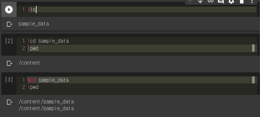
There are many differences in functionalities, but a key difference is that changes made by built-in line magics (%) are applied to the entire notebook environment. In contrast, ! command is only applicable to the subshell that is running the command.

It is easier to understand with examples. For example, if I want to move to a subdirectory sample_data. If I use !cd command to move to the subdirectory and print current directory with pwd, it shows that I am still in content directory. However, if I use the line magic %cd, I can keep myself in that directory.

Changing current directories

So, we just saw how to change current directories and print out current directory and subdirectories. They are not just used in Colab, but also frequently used in Ubuntu and MacOSX terminals. To summarize,

• !pwd command finds out the currently working directory
• !ls command finds out the current subdirectories
• %cd directory_to_move line magic moves current working directory.

Fetching & unzipping files from the Web

We sometimes want to download and open files, e.g., datasets, from the Web. In such cases, we can use the !wget command.

!wget url_to_the_file

Also, if you want to unzip those files, you can use either !unzip or !gunzip commands.

!unzip works with most conventional compressed files, e.g., .zip files, and gunzip works with .gz or .tgz files.

For more information on getting files from the Web and opening them, refer to this posting.

Default line magics

There are some “default” line magics that many people just run automatically before running other cells in Colab or Jupyter Notebooks. I learned to use them from the Practical Deep LEarning for Coders course provided by fast.ai.

• %matplotlib inline: ensures that all matplotlib plots are shown in the output cell, and will be kept in the notebook when saved.

• %reload_ext autoreload, %autoreload 2: reloads all modules before executing a new line. So when a module is updated, you don’t need to rerun the import command.

%matplotlib inline
%reload_ext autoreload
%autoreload 2

For a comprehensive list of line and cell magics, refer to the IPython documentation

In earlier postings, we figured out how to import files from Google Drive. By using the Google Drive file ID, we can import a single file, e.g., csv or txt file, from Google Drive.

However, in some cases, we might want to import more than one files. In such cases, it would be cumbersome to fetch file IDs of all the files that we want to import. There is a simple solution to that problem - mounting Google Drive. In this posting, let’s see how we can mount Google Drive and import files from your drive folder.

Mounting Google Drive

Assume that I want to import example.csv file under the folder data. Thus, the file is located at My Drive/data/example.csv.

The first step is mounting your Google Drive. Run below two lines of code and get the authorization code by loggin into your Google account. Then, paste the authorization code and press Enter.

from google.colab import drive
drive.mount("/content/drive")

If everything goes well, you should see the response “Mounted at /content/drive”

Double-check with the !ls command whether the drive folder is properly mounted to colab.

Importing files

Now you can import files from the Google Drive using functions such as pd.read_csv. Note that contents in your drive is under the folder /content/drive/My Drive/.

/content/drive/My Drive/location_of_the_file

For instance, if you want to open example.csv in /content/drive/My Drive/my_directory/, you can use below command using Pandas:

data = pandas.read_csv('/content/drive/My Drive/my_directory/example.csv')

Or, you could also use loadtxt() in NumPy.

data = numpy.loadtxt('/content/drive/My Drive/my_directory/example.csv', delimiter = ',')

For more information on decoding/parsing various file types, please refer to this posting

In previous posting, we went through downloading and importing datasets from the Web. With functions in NumPy and Pandas, we can import most datasets available on the Web, e.g., csv, tsv, spreadsheets, and txt files.

However, datasets, especially the large one, are provided in compressed formats such as .zip or .gz. In such cases, we should first unzip them to have access to the raw data. By taking advantage of terminal commands, we can conveniently hack this problem. Don’t be frightened with terminal commands, espeically if you are new to this. It is much easier and quicker than you think!

Finding the data source

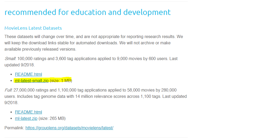
First and foremost, we need to know basic details of the data source. In this tutorial, let’s try downloading and importing a dataset from MovieLens. Among many datasets, let’s try Small MovieLens Latest Datasets recommended for education and development. The dataset that we want is contained in a zip file named ml-latest-small.zip.

As before, we first need to copy the url to the zip file. FYI, the url looks like this here: http://files.grouplens.org/datasets/movielens/ml-latest-small.zip. And if you download the zip file and open it, you will see that there are four csv files contained in a folder ml-latest-small.

Here, let’s try opening the ratings.csv file. The file has 100,836 instances with four attributes - userId, movieId, rating, and timestamp.

Download and unzip the compressed file

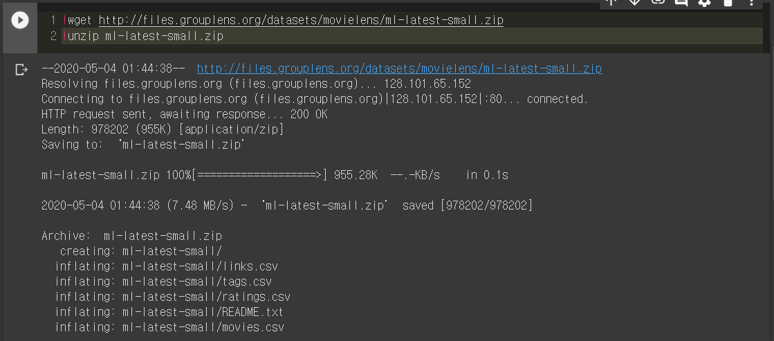
Then, now we can create a colab file and download and unzip the compressed file (ml-latest-small.zip). To download the compressed file (or any file in general), you can use the !wget command as below.

!wget url_to_the_zip_file

Then, you will need to unzip the compressed file to open the files contained in it. !unzip command will work for most files with extension .zip. However, for .gz or .tgz files, try the !gunzip command instead.

!unzip compressed_file_name.zip

Now check with the !ls command to check out whether the file is properly downloaded and unzipped. You should see ml-latest-small folder and ml-latest-small.zip file as below.

Import data

Finally, you can import the data using functions such as read_csv() or np.loadtxt() as we have seen in the previous posting.

In addition, if you want to move the working directory to the folder that you created while unzipping, you can use the %cd command (“change directory”).

%cd directory_name

In this posting, we have gone through the process of downloading, unzipping, and importing compressed datasets. Combining techniques outlined here and in other postings, you will be able to fetch most data to Colab with relative ease.

In previous postings, I outlined how to import local files and datasets from Google Drive in Colab.

• Importing CSV & JSON files
• Importing files from Google Drive

Nonetheless, in many cases, we want to download open datasets directly from the Web. In many cases, this will significantly reduce the time and effort. Also, as you will see, it is also space-efficient. While taking advantage of the hyperlinks, we can import virtually any data with few lines of code in colab.

Importing datasets from the Web

Many open datasets exist on the Web in the format of text files or spreadsheets. Using data import functions in the Pandas and NumPy libraries, it is very easy and convenient to import such files, given that you know the hyperlink.

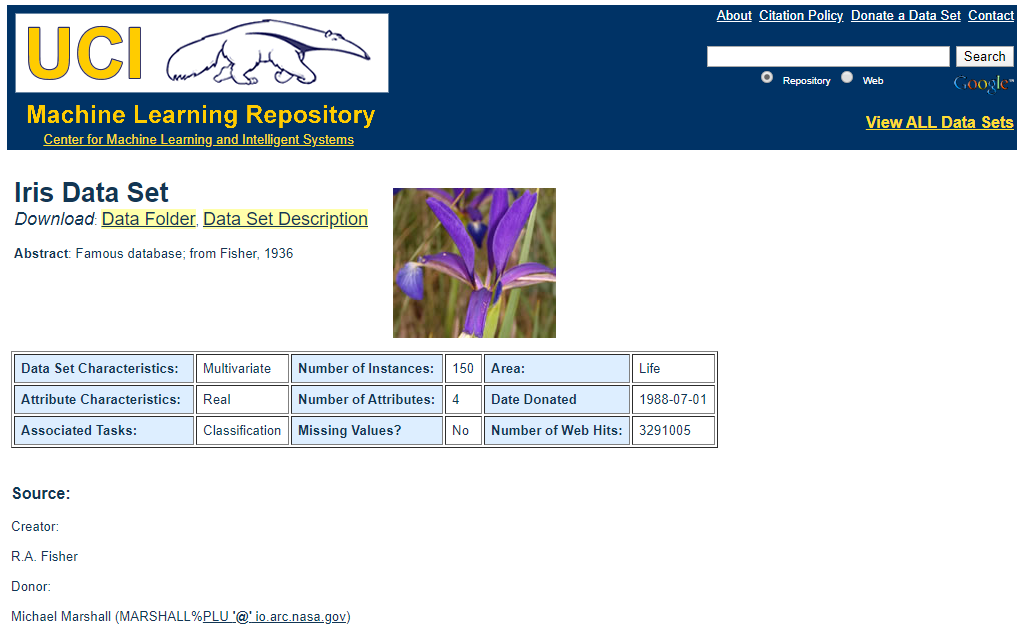
Suppose we want to import the famous Iris dataset from the UCI machine learning data repository.

The data is contained in the iris.data file. We do not need to download the file, just need the link address to the file as mentioned. You can just right click on it and copy the link. The link to the file should look like this: https://archive.ics.uci.edu/ml/machine-learning-databases/iris/iris.data

read_csv() function in Pandas

Since the data is delimited with commas (,), we can just paste the link in the first argument of read_csv() function. It will return a Pandas dataframe containing the content of the file.

df = pd.read_csv("url_to_the_file", header = None)

However, there are a few additional considerations when importing files as a Pandas dataframe in general. Below are a few of such considerations that you need to be aware of and general recommendations on how to take care of potential problems.

File extension

Files that you want to download can be in other file formats or not delimited with commas. In that case, consider using other functions such as pandas.read_table(), pandas.read_excel(), or pandas.read_json().

Delimiter

Another approach in dealing with non-comma-delimited datasets would be simply changing the delimiter. For instance, for tab separated datasets (i.e., TSV files), just set the sep argument to tab (“\t”).

Header (column names)

In some cases, column names are specified at the first row of the file. Then, do not set the header parameter to None as we did. Pandas will automatically infer the column names from the data and set them for the newly created dataframe.

Skipping rows

For some datasets, you would like to skip a few rows since they contain unnecessary information such as general descriptions about the data. In such cases, consider setting the skiprows parameter.

loadtxt() function in NumPy

Alternatively, we can also use np.loadtxt(). This had limited functionality compared to Pandas since we can only download text files, but can be efficient sometimes. np.loadtxt() will automatically convert the data into a NumPy array, which can be instantly used as inputs to many machine learning and deep learning models.

arr = np.loadtxt("url_to_the_file", delimiter = ",")

Again, below are some considerations for importing data with np.loadtxt() and troubleshooting guidelines.

Delimiter

This is the same problem with pd.read_csv(). For np.loadtxt(), manipulate the delimiter argument that has the same functionality as the sep argument in pd.read_csv().

Data types

Unlike Pandas dataframe, NumPy array has to keep all instances having same data types. In many cases where you have only numbers (floats, integers, doubles, …) in your dataset, this is not much of a problem. However, in our case, you can see that I have explicitly set the dtype as np.object to encode both String and Float data. Thus, if you want to manipulate the numerical data in our “object type” array, they have to be converted into numbers. This can be a significant problem for some cases, so please be mindful about data types!

In this posting, we gone through how to import data files to Colab. As mentioned, it is a very simple process given that you have the link to the file. However, some file extensions, such as zip files (.zip), cannot be imported just using functions such as pd.read_csv(). In the next posting, let’s see how we can deal with such files with Ubuntu terminal commands!