
Attention in Neural Networks - 23. BERT (2) Introduction to BERT (Bidirectional Encoder Representations from Transformers)
25 Jul 2020 | Attention mechanism Deep learning Pytorch BERT TransformerAttention Mechanism in Neural Networks - 23. BERT (2)
In the previous posting, we had a brief look at BERT. As explained, BERT is based on sheer developments in natural language processing during the last decade, especially in unsupervised pre-training and supervised fine-tuning. Thus, it is essential to review what have been done so far in those fields and what is new in BERT (actually, this is how most academic papers are written). I won’t be going into granular details of all important methods in the field. Instead, I will try to intuitively explain those that are essential in understanding BERT. If you want to learn more, you can read the papers that I have embedded the hyperlinks!
Unsupervised pre-training
As described in the previous posting, unsupervised word embedding models such as Word2vec and GloVe have become a crucial part in NLP. They represent each word as an n-dimensional vector, hence the name “word2vec.”
 [Mikolov et al. 2013]
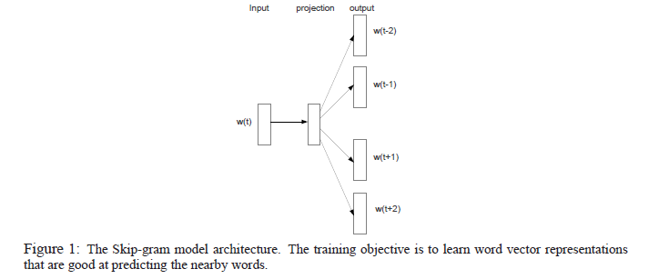
Those vectors are learned by a shallow neural network with a single hidden layer called the “projection layer.” The Skip-gram model, a type of word2vec, updates weights in the hidden layer while attempting to predict words close to the word of interest.
 [Mikolov et al. 2013]
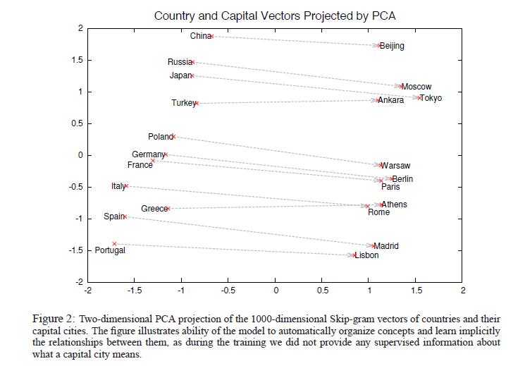
Since the learned vectors have the same dimensionality, they enable arithmetic operations between words. For instance, the similarity between words can be easily calculated using metrics such as cosine distance and relationships between them can be represented as equations as below.
\begin{equation} vec(“Montreal Canadiens”) - vec(“Montreal”) + vec(“Toronto”) = vec(“TorontoMaple Leafs”) \end{equation} \begin{equation} vec(“Russia”) + vec(“river”) = vec(“Volga River”) \end{equation} \begin{equation} vec(“Germany”) + vec(“capital”) = vec(“Berlin”) \end{equation}
Furthermore, they can be used as input features for various machine learning models to carry out downstream NLP tasks. For instance, it can be used to classify the sentiment the speaker is expressing at the point of speech (opinion mining/sentiment analysis), or find appropriate tags for a given image (image tagging). They are extended to represent not only words but also sentences and paragraphs in corpora.
However, they are not contextualized representations of words. That is, they are unable to model how the meanings of words can differ depending on linguistic contexts, i.e., modeling polysemy. Most words that we use frequently are highly polysemous. For instance, consider the use of word “bright” in two sentences below. In the first sentence, the word “bright” is synonymous to “smart” or “intelligent,” but in the second sentence, the word is antonymous to “dark.”
Jane was a bright student. The room was glowing with bright, purplish light pouring down from the ceiling.
However, it is difficult to model such context with unsupervised word embedding models such as word2vec and glove since they only look at word-level patterns. Therefore, contextualized word representation methods have been proposed recently to model such patterns. Embeddings from Language Models (ELMo) is one of the successfuly attempts to deeply contextualize word vectors.

ELMo consists of multiple bidirectional long short-term memory (LSTM) layers. However, instead of using just outputs from the top LSTM layer, a linear combination of the vectors stacked above each word is used for the downstream task. By doing so, they can jointly learn both syntactical and contextual features of words. My interpretation is that this is reminiscent of a hierarchy of convolutional neural network layers explained by Zeiler and Fergus (2014). This point was discussed in the earlier posting.
“Using intrinsic evaluations, we show that the higher-level LSTM states capture context-dependent aspects of word meaning (e.g., they can be used without modification to perform well on supervised word sense disambiguation tasks) while lower-level states model aspects of syntax (e.g., they can be used to do part-of-speech tagging).”
As a result, ELMo was able to improve the word representation significantly compared to existing methods and became one of state-of-the-art language models in 2018. However, Devlin et al. (2019) argued that ELMo is still “not deeply bidirectional” and feature-based, i.e., not fine-tuned for the downstream task. Therefore, they utilized the Transformer architecture that was already being used for fine-tuning language models such as OpenAI GPT. Now, let’s switch gears and have a look into supervised fine-tuning approaches.
Supervised fine-tuning
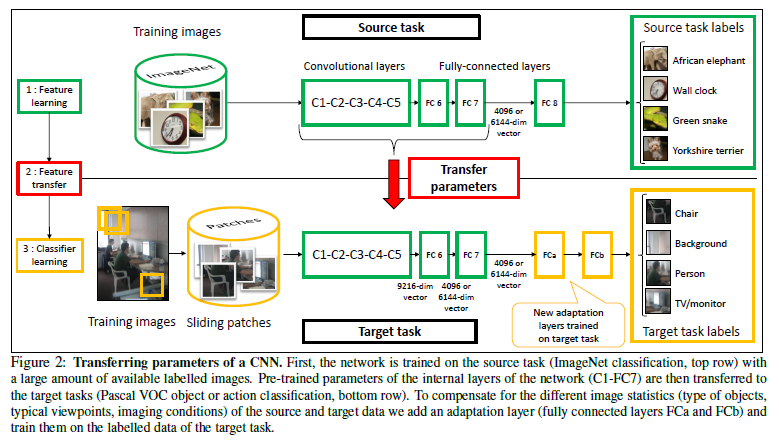
Unsupervised pre-training methods, contextualized or not, are somehow limited in terms of applicability since they are not aligned with downstream tasks. That is, they are not specificially tuned for a supervised task of interest. Therefore, NLP researchers started to borrow insights from computer vision, in which the concept of transfer learning has been en vogue. In practice, convolutional neural networks (CNN) are rarely trained from scratch nowadays. The image recognition field has standard, widely-accepted large-scale datasets such as CIFAR-10 and ImageNet. The images in those datasets are meticulously tagged and reliably verified by a number of studies. Established deep CNN architectures such as GoogleNet and VGG are pre-trained and publicly avaiable to anyone. Those pre-trained models show a remarkable capability for feature extraction in any given image. A classifier that is suitable for the downstream task, such as image segmentation and object detection, is placed on the top of the CNN and the CNN is retrained. For more information on transfer learning CNNs, please refer to this posting by CS231n (CNN for visual recognition) or Oquab et al (2013).
 [Oquab et al. 2013]
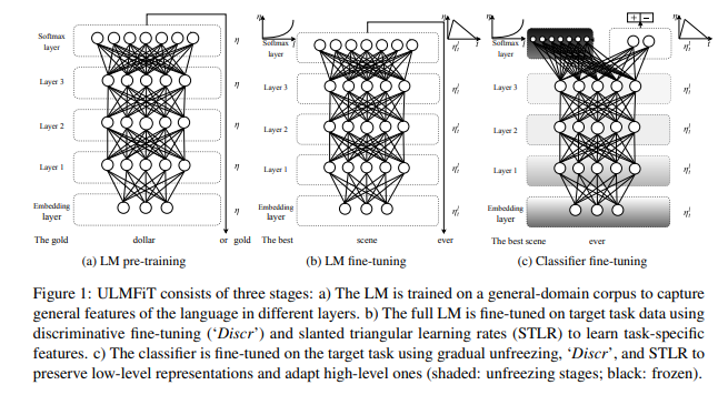
Motivated by the intuition in computer vision, Howard and Ruder (2018) proposed the Universal Language Model Fine-Tuning (ULMFiT). ULMFiT is one of the most successful attempts to apply inductive transfer learning for NLP tasks. It consists of two components - the language model (LM) and classifier. LM is a three-layer LSTM network followed after an embedding layer. First, LM is pre-trained on a general-domain corpus (usually large in scale) then fine-tuned on target task data. Finally, the classifier is fine-tuned on the target task.
 [Howard and Ruder 2018]
OpenAI’s Generative Pretrained Transformer (GPT) by Radford et al. (2018) takes a similar approach of generative pre-training followed by discriminative fine-tuning. Similar to ULMFiT, a standard LM is first pre-trained with an unsupervised corpus. Then, the overall model including the classifier is fine-tuned according to the target task. A novelty in GPT is that they use a multi-layer Transformer decoder, which is basically a variant of Transformer (Vaswani et al. 2017). Since different target tasks require different input structures, inputs are transformed depending on the target task. Below figure shows some examples of such transformations.
 [Radford et al. 2018]
A few days ago, OpenAI announced the introduction of GPT-3, which is the latest version of GPT. It is trained on about 400 billion encoded tokens, which amounts to around 570GB of compressed plaintext after filtering and 45TB before filtering. Further, it boasts about 175 billion parameters, which is 10x more than any previous non-sparse model. Arguably, the state-of-the-art of NLP in 2020 is Transformer-based transductive learning architectures.
Compared to GPT, BERT employs a similar, yet slightly different, mechanisms in pre-training and fine-tuning. In the next posting, let’s see how BERT is designed and implemented.
References
- Devlin et al. 2018
- Zeiler and Fergus 2014
- Kiros et al. 2015
- Le and Mikolov 2014
- Peters et al. 2018
- Howard and Ruder 2018
- Radford et al. 2018
- Brown et al. 2020

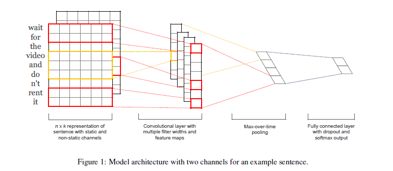 [Kim 2014]
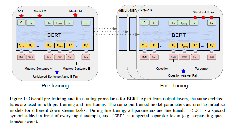 [Devlin et al. 2019]
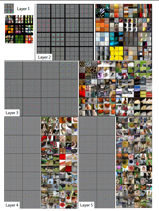 [Zeiler and Fergus 2014]
 [
[ [
[ [
[ [
[
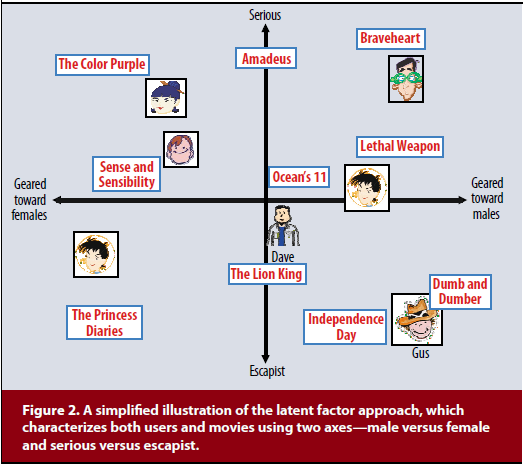
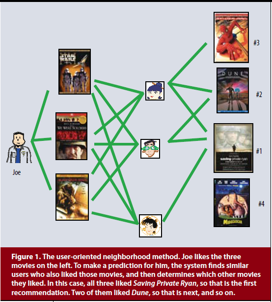 [Image source: Koren et al.]
 [Amazon's item-based recommendation]
 [Image source: Koren et al.]
![[Image Source]](https://en.wikipedia.org/wiki/File:Elmo_from_Sesame_Street.gif#/media/File:Elmo_from_Sesame_Street.gif)