In the previous posting, we implemented our first memory-based collaborative filtering system using theSurprise package in Python. In this posting, let’s see how we can improve the baseline k-NN model and try them to actually enhance the model’s performance on the MovieLens dataset.

Preparation

Prior to implementing the models, we need to install the Surprise package (if not installed already) and import it. For more information on installing and importing the Surprise package, please refer to this tutorial

from surprise import Dataset
from surprise import KNNBasic, BaselineOnly, KNNWithMeans,KNNWithZScore, KNNBaseline
from surprise.model_selection import cross_validate

Load a built-in dataset

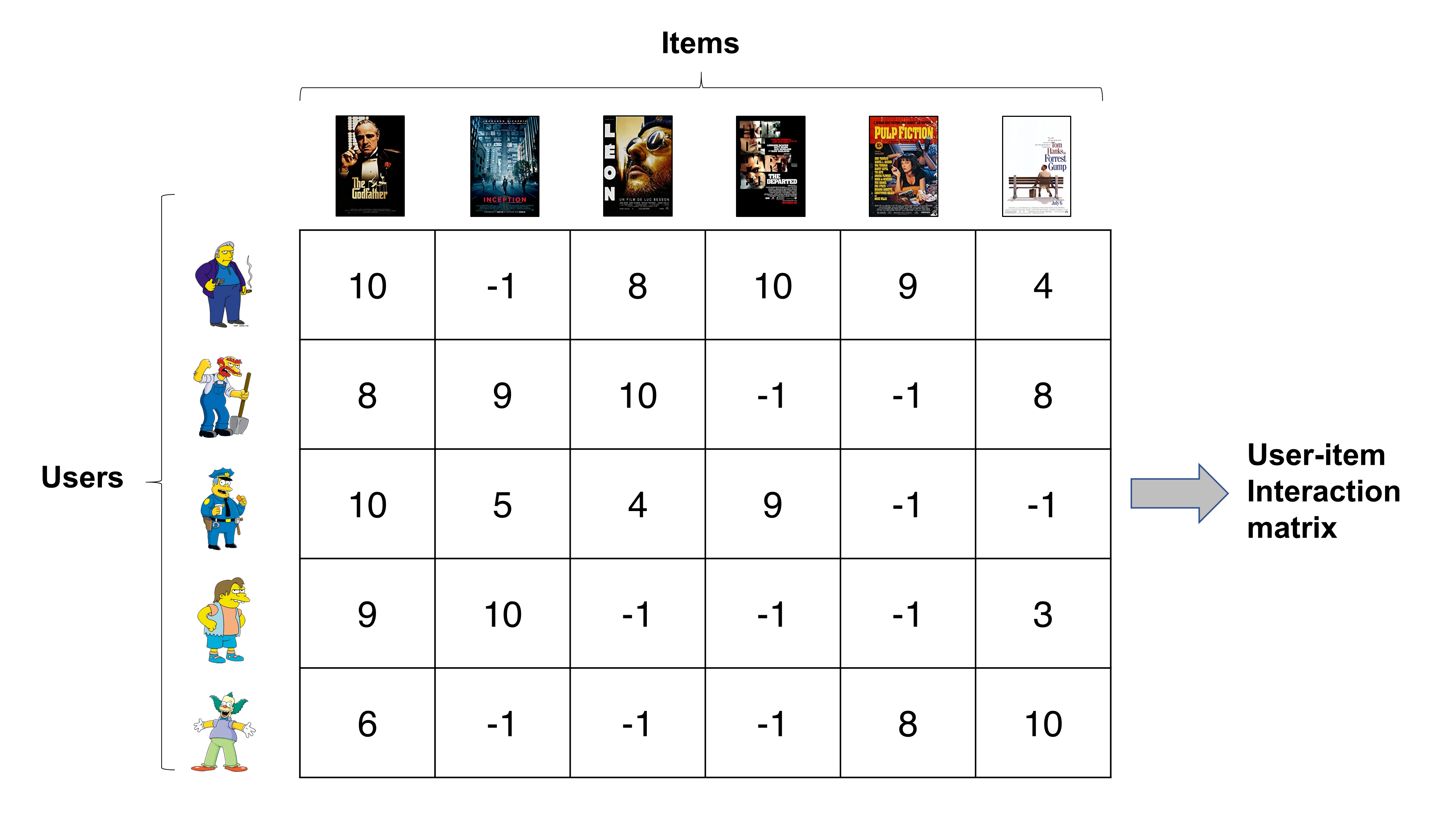
Let’s start with loading a built-in dataset. Again, let’s use the MovieLens dataset. For more details about the data, please refer to the previous postings.

dataset = Dataset.load_builtin()

Training & evaluation

Changing the number of neighbors (k)

Any variant k-NN algorithm involves aggregating information pertaining to a pre-defined number of neighbors. The notation for that pre-defined number is k. Hence, k is one of hyperparameters that can potentially influence performance of the machine learning model.

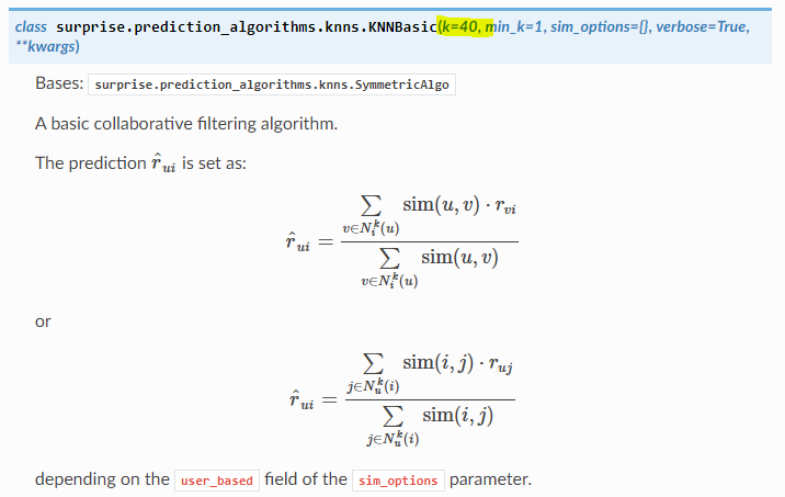
The default value of k is 40 for k-NN-inspired algorithms in Surprise. However, this number can be further fine-tuned for optimal performance. There is no one-size-fits-all solution for k, so it is recommended to find an optimal one with search schemes such as random search and grid search (Bergstra and Bengio 2012). Here, let’s try different values of from 10 to 100 and compare the results.

sim_options = {
    'name': 'MSD',
    'user_based': 'True'
}

cv_results = []
for k in range(1, 11):
  clf = KNNBasic(k= k*10, sim_options = sim_options)
  cv_results.append(cross_validate(clf, dataset, measures=['MAE'], cv=5, verbose=False))

for i in range(10):
  print("Average MAE for k = {} ".format((i+1)*10), cv_results[i]["test_mae"].mean())

It seems that setting k to around 30 yields relatively superior performance. However, differences in performances are not dramatic - we need other improvements to beat the baseline!

Average MAE for k = 10  0.7791384730857354
Average MAE for k = 20  0.7700308569739284
Average MAE for k = 30  0.770853160085353
Average MAE for k = 40  0.7729402525558153
Average MAE for k = 50  0.7756380474579305
Average MAE for k = 60  0.7774398619226626
Average MAE for k = 70  0.7807832701921905
Average MAE for k = 80  0.7821534570601616
Average MAE for k = 90  0.7850191446196909
Average MAE for k = 100  0.7856976099341807

Rating centering and normalization

Mean centering and normalization is a widely used feature transformation method in machine learning. In the recommendation context, the two methods convert individual ratings into a universal scailng. Even though we give the same ratings scale, e.g., 1-5 scale, how users perceive the absolute numbers in the scale can vary significantly. For instance, some users might be relatively “hard to please” compared to other users. Those users will consistently give lower ratings to most of the items that they have encountered. Therefore, mean centering subtracts the average of ratings that given by the user to every rating that the user has given. In addition, the Z-score normalization scheme considers “the spread” in the user’s rating scale.

The normalization can be conveniently implemented by using KNNWithZScore() instead of KNNBasic. It seems that the normalization yields a better performance, showing average test MAE of under 0.75. However, unfortunately, this is still not so satisfactory - the baseline estimator achieves similar performance.

sim_options = {
    'name': 'MSD',
    'user_based': 'True'
}

clf = KNNWithZScore(k=30, sim_options = sim_options)
cross_validate(clf, dataset, measures=['MAE'], cv=5, verbose=True)

                  Fold 1  Fold 2  Fold 3  Fold 4  Fold 5  Mean    Std     
MAE (testset)     0.7465  0.7479  0.7526  0.7455  0.7501  0.7485  0.0025  
Fit time          0.47    0.49    0.48    0.48    0.48    0.48    0.01    
Test time         3.55    3.48    3.57    3.50    3.62    3.55    0.05    
{'fit_time': (0.4673135280609131,
  0.486081600189209,
  0.48402929306030273,
  0.4768378734588623,
  0.48423147201538086),
 'test_mae': array([0.7464836 , 0.74794443, 0.75256676, 0.74552251, 0.75010478]),
 'test_time': (3.545177936553955,
  3.4846949577331543,
  3.5715558528900146,
  3.503652572631836,
  3.6209750175476074)}

Incorporating baseline estimates

Finally, we can consider incorporating baseline estimates. Essentially, this is combining the baseline estimator and k-NN in a single algorithm. The motivation behind this is similar to mean-centering. But here, the biases present in user- and item-levels, i.e., user and item effects, are simultaneously considered and estimated.

“For example, suppose that we want a baseline estimate for the rating of the movie Titanic by user Joe. Now, say that the average rating over all movies, $\mu$, is 3.7 stars. Furthermore, Titanic is better than an average movie, so it tends to be rated 0.5 stars above the average. On the other hand, Joe is a critical user, who tends to rate 0.3 stars lower than the average. Thus, the baseline estimate for Titanic’s rating by Joe would be 3.9 stars by calculating 3.7 − 0.3 + 0.5.” (Koren 2010)

The KNNBaseline() implements such model - the usage is identical to other k-NN models.

sim_options = {
    'name': 'MSD',
    'user_based': 'True'
}

clf = KNNBaseline(k=30, sim_options = sim_options)
cross_validate(clf, dataset, measures=['MAE'], cv=5, verbose=True)

The k-NN model with baseline estimates show test MAE of around 0.73. Finally, we were able to get a significant improvement over the vanilla k-NN and baseline model!

                  Fold 1  Fold 2  Fold 3  Fold 4  Fold 5  Mean    Std     
MAE (testset)     0.7349  0.7325  0.7333  0.7291  0.7370  0.7334  0.0026  
Fit time          0.63    0.66    0.67    0.66    0.67    0.66    0.02    
Test time         3.68    3.81    3.76    3.76    3.73    3.75    0.04    
{'fit_time': (0.6288163661956787,
  0.6560549736022949,
  0.6707336902618408,
  0.6592440605163574,
  0.6749463081359863),
 'test_mae': array([0.73487928, 0.73254759, 0.73325744, 0.72909275, 0.73704706]),
 'test_time': (3.682957410812378,
  3.811162233352661,
  3.7631664276123047,
  3.7610509395599365,
  3.7297961711883545)}

In this posting, we tried different schemes to improve the baseline estimator and vanilla k-NN. On top of these, there are of course many other ways to improve the model, including data processing and fine-tuning the hyperparamters. Let me know if you find better ways!

References

• Bergstra, J., & Bengio, Y. (2012). Random search for hyper-parameter optimization. The Journal of Machine Learning Research, 13(1), 281-305.
• Koren, Y. (2010). Factor in the neighbors: Scalable and accurate collaborative filtering. ACM Transactions on Knowledge Discovery from Data (TKDD), 4(1), 1-24.
• Ricci, F., Rokach, L., & Shapira, B. (2011). Introduction to recommender systems handbook. In Recommender systems handbook (pp. 1-35). Springer, Boston, MA.

In previous postings, we have gone through core concepts in memory-based collaborative filtering, including the user-item interaction matrix, similarity measures, and user/item-based recommendation. In this posting, let’s review those concepts while going through Python implementation using the Surprise package.

Preparation

Prior to implementing the models, we need to install the Surprise package (if not installed already) and import it. For more information on installing and importing the Surprise package, please refer to this tutorial

from surprise import Dataset
from surprise import KNNBasic, BaselineOnly
from surprise.model_selection import cross_validate

Load a built-in dataset

Let’s start with loading a built-in dataset. Here, let’s use the MovieLens dataset, which is one of the most widely used public datasets in the recommender systems field. The default setting for the load_builtin() function is downloading the MovieLens data. The data should be downloaded if not downloaded earlier.

dataset = Dataset.load_builtin()

Let’s see how many user and items are present in the data. There are 100,000 rating instances, and this is why this data is called ml-100k. FYI, MovieLens provides much larger datasets - you can check them out here.

ratings = dataset.raw_ratings

print("Number of rating instances: ", len(ratings))
print("Number of unique users: ", len(set([x[0] for x in ratings])))
print("Number of unique items: ", len(set([x[1] for x in ratings])))

Training & evaluation

Baseline estimator

Let’s start with the baseline algorithm that we had implemented in the previous posting. It is always good to have a baseline for benchmark - this gives you a yardstick of how good (or bad) your algorithm is.

clf = BaselineOnly()
cross_validate(clf, dataset, measures=['MAE'], cv=5, verbose=True)

It seems that the baseline algorithm shows the average mean absolute error of around 0.75 in a five-fold cross validation.

Estimating biases using als...
Estimating biases using als...
Estimating biases using als...
Estimating biases using als...
Estimating biases using als...
Evaluating MAE of algorithm BaselineOnly on 5 split(s).

                  Fold 1  Fold 2  Fold 3  Fold 4  Fold 5  Mean    Std     
MAE (testset)     0.7456  0.7479  0.7462  0.7521  0.7494  0.7482  0.0023  
Fit time          0.42    0.47    0.32    0.30    0.30    0.36    0.07    
Test time         0.11    0.23    0.10    0.10    0.18    0.14    0.05    
{'fit_time': (0.4205029010772705,
  0.47090888023376465,
  0.3164703845977783,
  0.3028404712677002,
  0.2975282669067383),
 'test_mae': array([0.7456069 , 0.74790715, 0.74621253, 0.75207455, 0.74940825]),
 'test_time': (0.10664844512939453,
  0.2300584316253662,
  0.10011959075927734,
  0.10106658935546875,
  0.18408536911010742)}

k-Nearest Neighbor (k-NN)

Let us move on to k-NN, which is a simple memory-based collaborative filtering algorithm. Now, you can implement your first memory-based recommender system!

Similarity options

An important parameter for k-NN-based algorithms in Surprise is sim_options, which describes options for similarity calculation. Using sim_options, you can set how similarity is calculated, such as similarity metrics. The default setting is using the Mean Squared Difference (MSD) to calculate pairwise similarity and user-based recommendations.

sim_options = {
    'name': 'MSD',
    'user_based': 'True'
}

You can change the similarity calculation method by converting the value mapped to the name key. Also, item-based recommender systems can be easily implemented by changing user_based value to False.

sim_options = {
    'name': 'pearson',
    'user_based': 'False'
}

User-based k-NN

Let’s try implementing a user-based k-NN model with the default similarity calculation method, i.e., MSD.

sim_options = {
    'name': 'MSD',
    'user_based': 'True'
}

clf = KNNBasic(sim_options = sim_options)
cross_validate(clf, dataset, measures=['MAE'], cv=5, verbose=True)

It seems that the average MAE is around 0.77 with a five-fold cross validation. This is actually worse than the baseline algorithm!

Computing the msd similarity matrix...
Done computing similarity matrix.
Computing the msd similarity matrix...
Done computing similarity matrix.
Computing the msd similarity matrix...
Done computing similarity matrix.
Computing the msd similarity matrix...
Done computing similarity matrix.
Computing the msd similarity matrix...
Done computing similarity matrix.
Evaluating MAE of algorithm KNNBasic on 5 split(s).

                  Fold 1  Fold 2  Fold 3  Fold 4  Fold 5  Mean    Std     
MAE (testset)     0.7727  0.7709  0.7686  0.7761  0.7776  0.7732  0.0033  
Fit time          0.34    0.39    0.39    0.41    0.42    0.39    0.03    
Test time         3.71    3.81    3.82    3.93    3.74    3.80    0.08    
{'fit_time': (0.3350553512573242,
  0.3878347873687744,
  0.39234137535095215,
  0.40755629539489746,
  0.4163696765899658),
 'test_mae': array([0.77267657, 0.77093624, 0.76855595, 0.77607487, 0.77755156]),
 'test_time': (3.7132723331451416,
  3.8124566078186035,
  3.8213281631469727,
  3.9288363456726074,
  3.736668348312378)}

Item-based k-NN (& changing the similarity metric)

Maybe the reason for a poor performance is wrong hyperparameters. Let’s try a user-based system with the pearson coefficient as a similarity metric.

sim_options = {
    'name': 'pearson',
    'user_based': 'False'
}

clf = KNNBasic(sim_options = sim_options)
cross_validate(clf, dataset, measures=['MAE'], cv=5, verbose=True)

However, to our frustration, the performance gets even worse with MAE over 0.80! Does this mean that k-NN performs actually worse than the baseline model, which is a dumb enough model?

Computing the pearson similarity matrix...
Done computing similarity matrix.
Computing the pearson similarity matrix...
Done computing similarity matrix.
Computing the pearson similarity matrix...
Done computing similarity matrix.
Computing the pearson similarity matrix...
Done computing similarity matrix.
Computing the pearson similarity matrix...
Done computing similarity matrix.
Evaluating MAE of algorithm KNNBasic on 5 split(s).

                  Fold 1  Fold 2  Fold 3  Fold 4  Fold 5  Mean    Std     
MAE (testset)     0.7984  0.8060  0.8006  0.8021  0.8081  0.8030  0.0036  
Fit time          1.46    1.39    1.57    1.51    1.52    1.49    0.06    
Test time         3.80    4.01    3.74    3.88    3.86    3.86    0.09    
{'fit_time': (1.4587411880493164,
  1.3949718475341797,
  1.5693511962890625,
  1.5131325721740723,
  1.5200302600860596),
 'test_mae': array([0.79836295, 0.80602847, 0.80057509, 0.80210933, 0.80808347]),
 'test_time': (3.799623966217041,
  4.005688190460205,
  3.7438101768493652,
  3.882983446121216,
  3.8566648960113525)}

Other considerations

Nonetheless, don’t be frustrated yet. Since k-NN is a relatively more sophisticated model than the baseline model, there are some other considerations that should be fully accounted for. In the following posting, let’s see how we can yield optimal performance with k-NN.

References

• Koren, Y. (2010). Factor in the neighbors: Scalable and accurate collaborative filtering. ACM Transactions on Knowledge Discovery from Data (TKDD), 4(1), 1-24.
• Ricci, F., Rokach, L., & Shapira, B. (2011). Introduction to recommender systems handbook. In Recommender systems handbook (pp. 1-35). Springer, Boston, MA.

So far, we have seen how users and items can be represented as vectors and users’ feedback records on items as entries in the user-item interaction matrix. Furthermore, using the matrix, we can calculate how two users or items are similar to each other. In this posting, let’s see how we can actually predict prospective ratings and recommend items by combining what we have reviewed so far.

User-based recommendation vs. Item-based recommendation

In the previous posting, we learned that users and items both can be represented as vectors and similarities can be calculated for each of user or item pairs. Therefore, item recommendation can be performed in two different ways, namely user-based and item-based.

User-based recommendation

For user-based recommendations, similarity calculation and neighborhood identification are performed among users. That is, we calculate similarity measures between users, i.e., user vectors in the interaction matrix, and identify $k$ nearest users. Then, we calculate the average rating among those $k$ users.

Note that the list of $k$ nearest users can differ based on which item that we want to estimate ratings for. This is because some users could have not rated the item of interest. For instance, assume that we want to predict the rating on The departed by Krusty. Let’s assume Willie is the most similar user to Krusty. However, Willie did not watch The departed and rate the movie as a result. Thus, we need to neglect Willie’s record and find other users that is both similar to Krusty and have watched and rated the movie.

Once $k$-nearest users satisfying the both conditions are found, the rating can be estimated by simply averaging the neighbors’ ratings that are given to the item of interest.

\begin{equation} \hat{r_{ui}} = \frac{1}{|N_i(u)|} \displaystyle\sum_{v \in N_i(u)} (r_{vi}) \end{equation}

In some practical cases, simply averaging can be insufficient. Therefore, many improvements such as weighing the ratings based on similarity metrics and normalizing the ratings have been proposed. However, this is also contingent upon the context - it is important to understand the problem and data before choosing/improving your averaging scheme.

Item-based recommendation

Instead of finding similar users and averaging ratings on the item of interest, item-based recommendation tries to find similar items to the item of interest. Then, we average the ratings to those items given by the user. Again, we cannot include the items that have not been previously rated by the user to the neighborhood. Once the $k$-nearest items are retrieved, we can average the ratings using the following equation.

\begin{equation} \hat{r_{ui}} = \frac{1}{|N_u(i)|} \displaystyle\sum_{j \in N_u(i)} (r_{uj}) \end{equation}

Here, similar improvements such as weighting and normalization can be employed.

User- or Item-based, which one is better?

Traditionally, user-based recommendation methods were employed in practice. However, they were reported to have severe scalability and sparsity issues, especially with very large datasets that are prevelant nowadays. Hence, large-scale web applications such as Amazon.com started to move onto item-based collaborative filtering (Sarwar et al. 2001, Linden et al. 2003). In my opinion, both are methodologically sound, strong baselines with appealing features such as convenient implementation and explainability of the results. Thus, it would be meaningful to employ both methods and compare the results with more sophisticated methods that we are going to have a look in the following postings.

References

• Linden, G., Smith, B., & York, J. (2003). Amazon. com recommendations: Item-to-item collaborative filtering. IEEE Internet computing, 7(1), 76-80.
• Ricci, F., Rokach, L., & Shapira, B. (2011). Introduction to recommender systems handbook. In Recommender systems handbook (pp. 1-35). Springer, Boston, MA.
• Sarwar, B., Karypis, G., Konstan, J., & Riedl, J. (2001, April). Item-based collaborative filtering recommendation algorithms. In Proceedings of the 10th international conference on World Wide Web (pp. 285-295).

In the previous posting, we went through how users and items can be represented as vectors and their interaction records are expressed as a matrix. Then, we have seen how the distance (similarity) between users (or items) can be computed using vector representations. In this posting, let’s look deeper into how the distances can be calculated using diverse schemes.

User-item interaction matrix revisited

Let’s go back to the movie recommendation system with five users Tony, Willie, Wiggum, Nelson, and Krusty. They rated six movies, which are The Godfather, Inception, Leon, The Departed, Pulp Fiction, and Forrest Gump, on a 10-point scale.

In the previous posting, we have discussed how to calculate the distance between two users using the Manhattan distance metric. Manhattan distance is basically the sum of the absolute values from element-wise subtraction. From the matrix above, we just need to retrieve elements in the corresponding rows and perform necessary operations on them, after excluding unobserved entries. For instance, the Manhattan distance between Tony and Krusty can be calculated as below.

\begin{equation} |v_{tony} - v_{krusty}| = |(4, -1, -1, -1, 1, 6)| = 11 \end{equation}

The distance between items can be calculated in a similar manner. We just need to use corresponding columns, instead of rows in this case. We can see that the movie The Godfather is more close to the movie Leon than the movie Forrest Gump.

\begin{equation} |v_{the \ godfather} - v_{forrest \ gump}| = |(6, 0, 6, -4)| = 16 \end{equation}

\begin{equation} |v_{the \ godfather} - v_{leon}| = |(2, -2, 6)| = 10 \end{equation}

Correlation-based similarity

Correlation-based similarity is another common-sensical way to measure the proximity between users or items. Remember that collaborative filtering is also known as “people-to-people” correlation method? We can calculate how two users (or items) correlate with each other using correlation coefficients. The most widely used correlation metric is the Pearson correlation coefficient. Pearson correlation similarity between two users u and v can be calculated as follows:

\begin{equation} corr(u, v) = \frac{\displaystyle\sum_{i \in I}(r_{ui} - \bar{r_u})(r_{vi} - \bar{r_v})}{\sqrt{\displaystyle\sum_{i \in I}(r_{ui} - \bar{r_u})^2 \displaystyle\sum_{i \in I}(r_{vi} - \bar{r_v})^2}} \end{equation}

, where $I$ is the items commonly rated by users u and v, $r_{ui}$ and $r_{vi}$ are ratings given to the item $i$ by u and v respectively. Finally, $\bar{r_u}$ and $\bar{r_v}$ are the average ratings given by u and v respectively.

Image source

The numerator of the metric measures how the ratings by the two users tend to vary in a similar fashion to each other. Hence, this part is also known as covariance. The denominator scales this measure, confining its values between -1 and 1.

Mean squared diffrence (MSD)

MSD is another popular similarity metric. It is the inverse of the mean squared difference of ratings between users u and v. Note that it is expressed as an inverse of the difference to indicate how similar two users (items) are. Furthermore, MSD is similar to the Pearson Correlation coefficient since it also tries to capture normalized covariant pattenrs between user ratings. Nonetheless, MSD does not take into account negative correlation since it can only take positive values.

\begin{equation} MSD(u, v) = \frac{|I|}{\sqrt{\displaystyle\sum_{i \in I}(r_{ui} - r_{vi})^2}} \end{equation}

Other similarity metrics

So far, we have seen three widely used similarity (distance) metrics. However, there are many other metrics such as cosine similarity, Jaccard similarity, and Spearman rank correlation. As in any other data mining problem, I should say there is no one-size-fits-all method to measure the level of similarity. Furthermore, you can define your own similarity function that suits the problem context! All metrics have their own pros and cons and you can be creative to complement limitations of existing approaches. In the following posting, let’s see how we can use calculated similarity metrics to recommend items to a user.

References

• Ricci, F., Rokach, L., & Shapira, B. (2011). Introduction to recommender systems handbook. In Recommender systems handbook (pp. 1-35). Springer, Boston, MA.
• Sarwar, B., Karypis, G., Konstan, J., & Riedl, J. (2001, April). Item-based collaborative filtering recommendation algorithms. In Proceedings of the 10th international conference on World Wide Web (pp. 285-295).

In the previous posting, we reviewed key ideas of and intuition behind the memory-based (a.k.a neighborhood/heuristic) methods. The crux of most memory-based methods are the concept of “neighborhood,” which is a set of instances that are close, or similar, to each other. Thus, in this posting, let’s see how we measure and compute the level of similarity between users and items.

User-item interaction matrix

As in most data mining problems, it is convenient to think users and items as vectors in a user-item interaction matrix. Assume that we are building a movie recommender system. We just started to build it, so there are only five users now, who are Tony, Willie, Wiggum, Nelson, and Krusty (BTW, these are my favorite characters in Simpsons. Don’t ask why lol). They rated six movies, which are The Godfather, Inception, Leon, The Departed, Pulp Fiction, and Forrest Gump, in a 10-point scale. Once we get data regarding their ratings information, we need to record such data in some consistent format. The most common approach to record such information is creating a table using spreadsheets such as below.

Each row pertains to a user and each column is for a movie. And each element in the table shows rating information by a user in the corresponding row of a movie in the corresponding column. For instance, the number in the first row, third column is Tony’s ratings of the movie Leon, which is 8 out of 10. And the number in the fourth row, sixth column is Nelson’s rating for the movie Forrest Gump. Now, the rating information indicates how users interacted with movies, i.e., items. Hence, user-item interaction matrix is essentially a fancy name for this table. So don’t be afraid of technical terms “interaction” or “matrix” - even you can create a small user-item interaction matrix using Excel or Google Sheets.

Missing values, sparsity, and implicit/explicit feedbacks

If you have a second look at the table above, you will see that some entries have negative values, i.e., -1. This is where there is no rating information. In other words, the user has not rated the item. For example, Tony hasn’t rated the movie Inception and Wille hasn’t rated the movies the Departed and Pulp Fiction. I set the value to -1 to distinguish from ratings that have positive values. You can use any other value, given that it is distinguished from ratings.

If there are much more missing values than positive values, we have a sparsity problem. The matrix is so sparse that it is difficult to derive meaningful collaborative patterns from it. The sparsity problem is prevalent in practice. In many cases, it is difficult to obtain explicit feedbacks such as ratings. For instance, only a fraction of purchasers at Amazon.com leave ratings and reviews. Even though we know they purchased an item, we don’t know whether they were satisfied with the item or not. And that is why they ask us to leave ratings after the purchase as below. But to be honest, I rarely leave reviews. Sorry! But there are many people like me, exacerbating the sparsity problem.

Thus, in many practical cases, we rely on implicit feedbacks, which are subtle cues that indicate the user’s preference. The number of revisits to a movie page and search history can be good examples of implicit feedbacks. But here, let’s just focus on explicit feedbacks, since they are most straightforward to model. We can come back to implicit feedbacks after we familiarize with explicit feedbacks.

Users and items as vectors

Now, let’s come back to the point that users and items can be represented as vectors. For instance, a vector for Tony in the matrix is $v_{tony} = (10, -1, 8, 10, 9, 4)$ and a vector for Krusty the clown is $v_{krusty} = (6, -1, -1, -1, 8, 10)$. Similarly, vectors for movies can be obtained by column-wise slicing of the matrix. The key advantage of doing this is that we can perform various arithmetic operations and optimization tasks.

Image source

A simplest way to obtained a distance between two users (or items) is to subtract one vector from another and sum the absolute values. This is called Mahattan distance. The intuition behind is pretty self-explanatory. The absolute value of element-wise subtraction is the difference in ratings to that movie by both users. For instance, since Tony gave 10 scores to The Godfather and Krusty gave 6, the absolute difference is 4. In more mathematical terms, the distance in The Godfather dimension is 4. Therefore, we are summing up distances in each dimension, i.e., each movie, to obtain an aggregated distance for all movies.

\begin{equation} |v_{tony} - v_{krusty}| = |(4, -1, -1, -1, 1, 6)| = 11 \end{equation}

One thing to note is that we are only considering the movies both Tony and Krusty gave ratings to, i.e., The Godfather, Pulp Fiction, and Forrest Gump. We cannot calculate distance for the movie that either of them did not give ratings to. This is why high sparsity can be a thorny problem - more missing values implies less dimensions can be taken into account.

As mentioned, the Manhattan distance is one of the simplest method to calculate the distance. I used it in this posting to provide intuitiion to the concept of similarity and distance. Of course there are many distance metrics that are more sophisticated than that. We will see them in the next posting!

References

• Ricci, F., Rokach, L., & Shapira, B. (2011). Introduction to recommender systems handbook. In Recommender systems handbook (pp. 1-35). Springer, Boston, MA.
• Koren, Y., Bell, R., & Volinsky, C. (2009). Matrix factorization techniques for recommender systems. Computer, 42(8), 30-37.