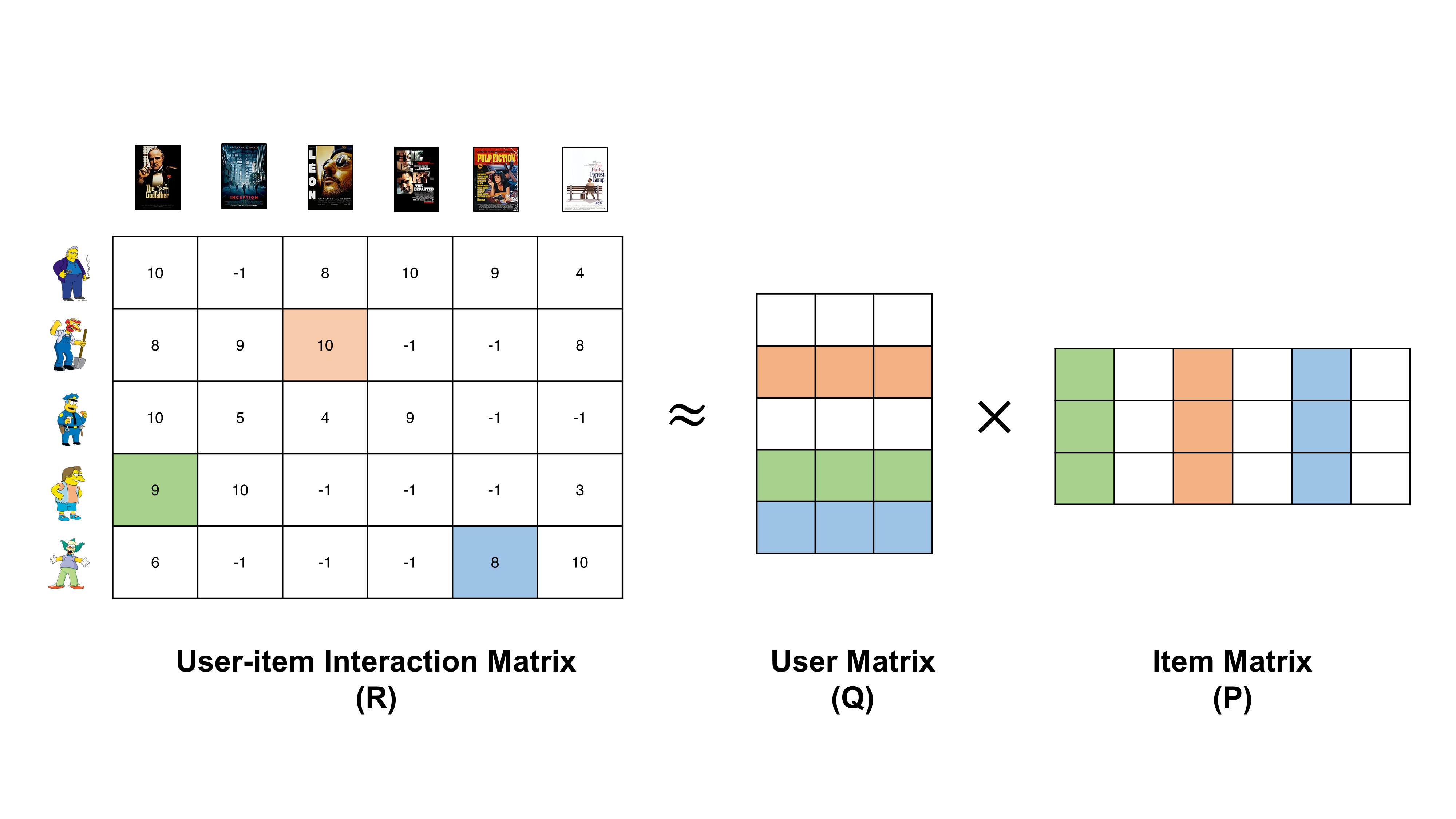
So far, we have studied the overall matrix factorization (MF) method for collaborative filtering and two popular models in MF, i.e., SVD and SVD++. I believe now we know how MF models are designed and trained to learn correlation patterns between user feedback behaviors. In this posting, without further ado, let’s try implementing MF in Python using Surprise.

Data preparation

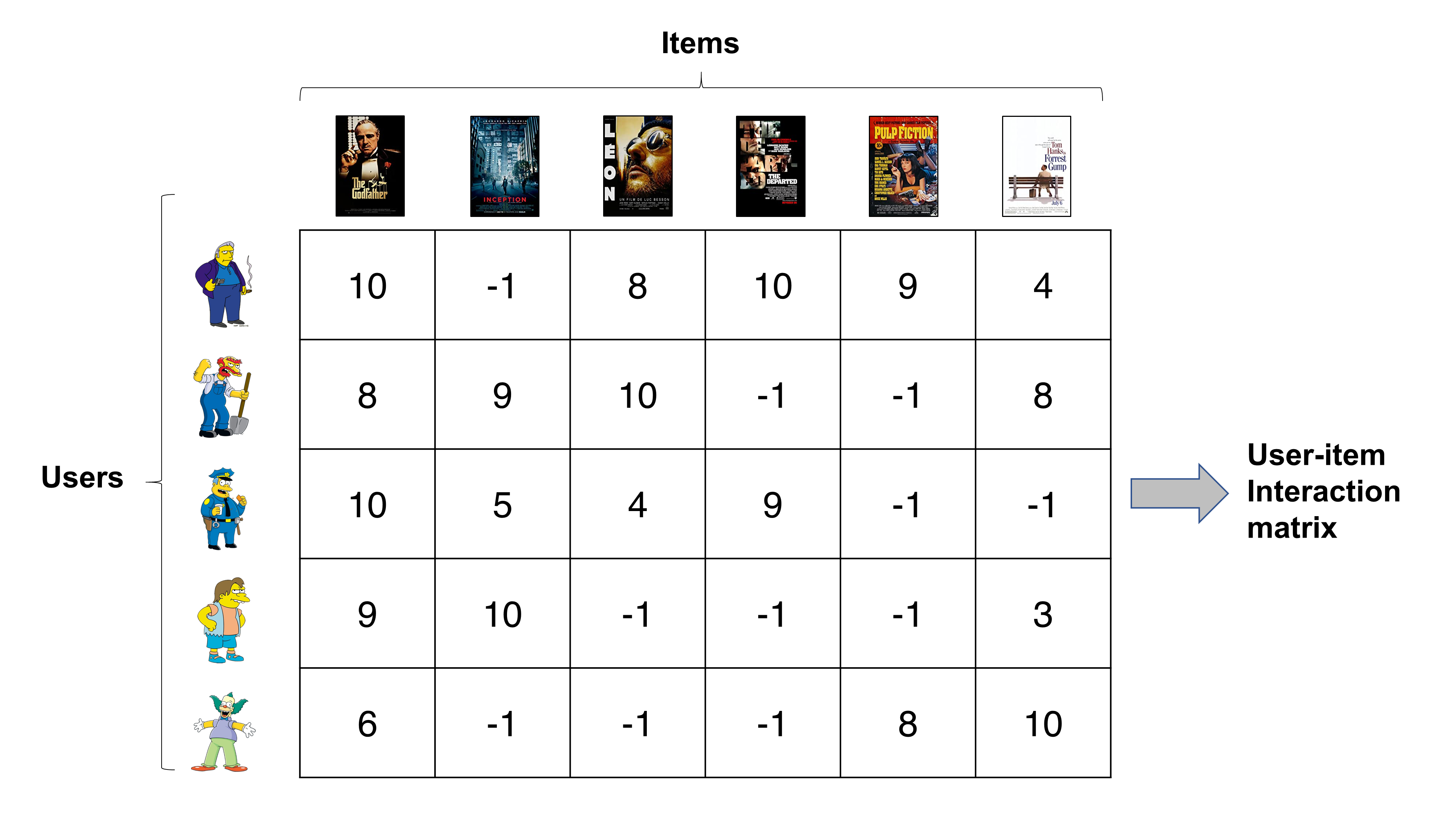
Let’s load the MovieLens dataset, which was used in prior postings. For more information on importing and loading the built-in dataset, please refer to the previous posting

from surprise import Dataset
dataset = Dataset.load_builtin()

Implementing SVD

Training and evaluating SVD is very straightforward, similar to implementing the k-NN and baseline estimator when using Surprise. We just need to define the model with SVD() - Surprise will take care of most of the things for us. Again, let’s try five-fold cross-validating.

from surprise import SVD

clf = SVD()
cross_validate(clf, dataset, measures=['MAE'], cv=5, verbose=True)

To our dismay, SVD does not seem to do extremely well in this case. In fact, it shows test MAE scores slightly above 0.73. This is on a par with k-NN with the baseline estimator that we have implemented in this posting.

Evaluating MAE of algorithm SVD on 5 split(s).

                  Fold 1  Fold 2  Fold 3  Fold 4  Fold 5  Mean    Std     
MAE (testset)     0.7398  0.7365  0.7410  0.7353  0.7378  0.7381  0.0021  
Fit time          4.99    5.03    5.00    5.03    4.99    5.01    0.02    
Test time         0.14    0.22    0.14    0.22    0.14    0.17    0.04    
{'fit_time': (4.988102436065674,
  5.031152009963989,
  4.997517824172974,
  5.02509069442749,
  4.992721796035767),
 'test_mae': array([0.7398014 , 0.73648218, 0.74099867, 0.73526241, 0.73778967]),
 'test_time': (0.14092421531677246,
  0.2161257266998291,
  0.13858461380004883,
  0.21789216995239258,
  0.1449432373046875)}

But again, don’t be discouraged too early. Remember the first k-NN model that we implemented actually performed worse than the baseline estimator? There might be some things that we could do here as well.

Parameter tuning with grid search

Remember the accuracy scores fluctuated as we changed $k$ when implementing k-NN models? We also learned that $k$ is a hyperparameter that should be determined prior to training a machine learning model. We can do a similar thing here, but with different hyperparameters.

From my experience, two of the most important hyperparameters when running the stochastic gradient descent (SGD) algorithm are learning rate and number of epochs. Learning rate is the value $\gamma$ that is used to update the parameters and number of epochs counts how many parameter updates that the model is to carry out. The default settings for learning rate and number of epochs are 0.005 and 20, respectively. However, this might not be the optimal setting for our data.

Hence, let’s try grid search, which is an optimization scheme trying all possible combinations of specified hyperparameter choices. For more information on hyperparameter optimization, please refer to this Wikipedia article. Below code runs grid search using five-fold cross validation and prints out the best MAE and hyperparameter combinations that yielded the best score. Specifically, we try 16 (4 by 4) possible combinations of two parameters:

• learning rate: (5, 10, 20, 30)
• number of epochs: (.0025, .005, .001, .01)

from surprise.model_selection import GridSearchCV

grid = {'n_epochs': [5, 10, 20, 30], 
        'lr_all': [.0025, .005, .001, .01]}

gs = GridSearchCV(SVD, grid, measures=['MAE'], cv=5)
gs.fit(dataset)

print(gs.best_score['mae'])
print(gs.best_params['mae'])

However, again to our dismay, the result has not improve significantly - it shows MAE of around 0.73.

0.7374588888101046
{'n_epochs': 10, 'lr_all': 0.01}

SVD++

Even after tuning parameters, SVD didnt’s show superior performance to other models. Now, let’s try out SVD++, which is known to improve SVD. Fortunately, implementing SVD++ is very convenient - just replace SVD() with SVDpp().

from surprise import SVDpp

clf = SVDpp()
cross_validate(clf, dataset, measures=['MAE'], cv=5, verbose=False)

Finally, we are able to get results that are better than baselines. SVDpp shows test MAE around 0.72, which is slightly lower than scores from k-NN and SVD.

{'fit_time': (163.75455975532532,
  163.009015083313,
  163.31932163238525,
  163.62001395225525,
  163.37179136276245),
 'test_mae': array([0.72057974, 0.71956503, 0.72017268, 0.71820603, 0.72156721]),
 'test_time': (4.107621908187866,
  3.976837635040283,
  3.9505584239959717,
  3.752680778503418,
  3.8454060554504395)}

Additional considerations…

Although SVD++ shows better performance to other models that we have seen so far, it is not always desirable to use SVD++. If you have run the code in this posting, you would have noticed that SVD++ takes considerably longer time to train, compared to the naive SVD. Also, MF models, which are more complex than k-NN or baseline models, require more hyperparameters to tune for optimal performance. Finally, there is the problem of interpretability (or explainability or transparency), which is a critical issue for practical usage. It is often risky to blindly deploy the most accurate model without assessing its inner workings. Moreover, in general, more accurate models tend to be less interpretable, i.e., interpretability-accuracy tradeoff.

For such reasons, I oftentimes use very simple and light models for practical applications such as logistic regression and rule-based methods. And the recommender systems field is not an exception - it might be better to use simple memory-based models than fancy models such as SVD++ or neural net-based models, although the latter shows superior test accuracy. Unfortunately, there is no clear-cut answer to this - you should try as many approaches as possible and come up with an optimal solution that satisfies problem contraints, e.g., available computing resources and the need for interpretations.

References

• Koren, Y., Bell, R., & Volinsky, C. (2009). Matrix factorization techniques for recommender systems. Computer, 42(8), 30-37.
• Ricci, F., Rokach, L., & Shapira, B. (2011). Introduction to recommender systems handbook. In Recommender systems handbook (pp. 1-35). Springer, Boston, MA.

In the previous posting, we learned how vanilla matrix factorization (MF) models work for the rating prediction task. In this posting, let’s see how different variants of MF are optimized for performance.

Basic optimization scheme

As briefly discussed earlier, virtually every MF model essentially tries to minimize the difference between observed and predicted rating. And predicted rating is the dot product of corresponding user ($q_u$) and item ($p_i$) latent factors. Therefore, we get the basic optimization scheme:

\begin{equation} minimize \sum_{u, i} difference(r_{ui} - q_{u}^{T}p_{i}) \end{equation}

The difference can be calculated using various metrics such as mean squared error or mean absolute error. In the rest of this posting, let’s see how this simple optimization scheme can be improved for a better prediction performance.

SVD

SVD, or FunkSVD since it was first popularized by Simon Funk, is one of the pioneering models in MF for collaborative filtering. At first, many (including me) would be curious to see the relation to the singular value decomposition (SVD) of a square matrix in linear algebra. However, the SVD model in MF does not bear much resemblance to SVD commonly known in linear algebra. In fact, this was what left me very much confused in the outset. I won’t go into the details here, but please refer to this posting at freecodecamp.com for more information. In short, if you don’t know much about SVD, it doesn’t matter, and if you are familar with SVD in linear algebra, don’t expect to see the same thing here!

Objective function

It has two distinct features from the vanilla MF that we have seen earlier - (1) user/item biases and (2) regularization terms. First, the baseline estimates for users and items are incorporated as user ($b_u$) and item biases ($b_i$). Thus, the estimated ratings is:

\begin{equation} \hat{r_{ui}} = \mu + b_u + b_i + q_{u}^{T}p_{i} \end{equation}

where $\mu$ is the overall average rating. Also, the squared error is regularized to prevent overfitting to a user and/or item. By adding the two to the optimization objective, SVD generally demonstrates a superior performance over validation test data.

\begin{equation} minimize \sum_{u, i} (r_{ui} - (\mu + b_u + b_i + q_{u}^{T}p_{i}))^2 + \lambda(b_u^2 + b_i^2 + {\parallel q_u \parallel}^2 + {\parallel p_i \parallel}^2) \end{equation}

Learning

A simple stochastic gradient descent (SGD) algorithm can be applied to update the parameters and learn the patterns. Since the objective is to minimize the difference between the predicted and actual ratings, parameters ($b_u, b_i, q_u, p_i$) are updated by moving towards the opposite direction of the computed gradient. This would be easier to understand if you grasp the intuition behind SGD in machine learning in general. Once the error term $e_{ui} = r_{ui} - \hat{r_{ui}}$ is computed, parameters are updated following the below scheme.

\begin{equation} b_u \leftarrow b_u + \gamma (e_{ui} - \lambda b_u)
\end{equation} \begin{equation} b_i \leftarrow b_i + \gamma (e_{ui} - \lambda b_i)
\end{equation} \begin{equation} q_u \leftarrow q_u + \gamma (e_{ui} - \lambda q_u)
\end{equation} \begin{equation} p_i \leftarrow p_i+ \gamma (e_{ui} - \lambda p_i)
\end{equation}

$\lambda$, just like $\gamma$ are hyperparameters that should be determined before training the model. As we have seen, a higher level of $\gamma$ will regularize the parameters and suppress overfitting. Whereas, $\lambda$ is used to control the size of each step in the parameter update. Both should be set to optimal values meticuously using tuning methods such as grid search.

SVD++

SVD is a great choice when we have reliable and sizable explicit feedback information from users such as ratings. Nevertheless, in many cases, we have much richer implicit information such as search history, page visits, likes and sharing, and bookmarks. Such information can be effectively used to improve the learning process whether or not explicit feedback is abundant or not. SVD++ is one of the methods that exploits such information with a slight modification in SVD.

To model the implicit feedback, an additional term is added to $q_u$ to represent the user. The revised user factor is as below.

\begin{equation} q_u + {|R(u)|}^{-1/2} + \sum_{j \in R(u)} y_j \end{equation}

where $R(u)$ is the set of items rated by the user $u$ and $y_j$ is anothger factor vector to represent each item in $R(u)$. Hence, to represent a user, SVD++ combines the user factor learned from explicit ratings ($q_u$) and implicit information from items that the user has rated (or searched, shared, visited, etc.) previously ($R(u)$). In other words, it combines the model-based and memory-based approaches in a single equation. As a result, it generally shows superior performances to both SVD and memory-based models such as k-NN.

According to the changes in the user representations, the equation for rating estimation is modified as follows:

\begin{equation} \hat{r_{ui}} = \mu + b_u + b_i + (q_{u} + {|R(u)|}^{-1/2} + \sum_{j \in R(u)} y_j)^{T}(p_{i}) \end{equation}

The parameters can be updated using SGD, similar to the learning scheme for SVD. Just note that we have additional parameters to run, i.e., $y_j$’s, for implicit information.

References

• Funk, S. (2006) Netflix Update: Try This at Home. (https://sifter.org/~simon/journal/20061211.html)
• Koren, Y. (2008, August). Factorization meets the neighborhood: a multifaceted collaborative filtering model. In Proceedings of the 14th ACM SIGKDD international conference on Knowledge discovery and data mining (pp. 426-434).
• Koren, Y., Bell, R., & Volinsky, C. (2009). Matrix factorization techniques for recommender systems. Computer, 42(8), 30-37.
• Ricci, F., Rokach, L., & Shapira, B. (2011). Introduction to recommender systems handbook. In Recommender systems handbook (pp. 1-35). Springer, Boston, MA.

In the previous posting, we have briefly gone through the Netflix Prize, which made Matrix Factorization (MF) methods famous. In this posting, let’s dig into MF methods.

MF as a family of methods

As described earlier, MF for recommendation is a loosely defined term to denote methods that decomposes a rating matrix for collaborative filtering. Hence, it could be regarded as a family of methods involving matrix decomposition procedure. However, methods that are categorized as MF show some common properties. In the remainder of this posting, let’s see what those properties are.

MF basics

User-item interaction matrix revisited

We return to the user-item interaction matrix again. To recap, user-item interaction matrices generally lists users and items in rows and columns, respectively. Then, the interaction records between them are represented as corresponding elements in the matrix. Below matrix is an example of an interaction matrix in a movie recommender engine. Rows in the matrix shows how each user rated items (movies) and columns show how each movie is rated by all users. For more information on user-item interaction matrices, please refer to this posting.

Decomposition of the user-item interaction matrix

After the user-item interaction matrix is generated, it has to be decomposed into two matrices, which are the user matrix ($Q$) and item matrix ($P$). The user and matrices contain descriptions of users and items respectively with learned features. Those features are determined by the developer as they would be in content-based recommender systems. They are intrinsic features of users and items that are unearthed by the algorithm - this is also the reason why MF models are also known as latent factor models.

The low-dimensional, latent features are characterized by the algorithm such that they capture correlational patterns in previous user-item interaction records. Therefore, when properly estimated, the user and item matrices can precisely approximate previous user-item interaction patterns and ultimately, used to predict unknown records in the rating matrix. Take the example above of decomposing movie rating matrix. Here, the number of latent features is set to 3 - this is an arbitrary number set by the developer (generally set to a value significantly smaller than the number of users or items). Each row of $Q$ ($q_i$) describes each user and each column of $P$ ($p_j$) describes each movie. And the dot product of $q_i$ and $p_j$ is the estimated rating by the corresponding user to the movie. In a succint equation form,

\begin{equation} r_{ij} = q_{i}p_{j} \end{equation}

The second row of $Q$ represents the second user, i.e., Willie, and the third column of $P$ represents the third item, i.e., Leon. Hence, the dot product of the two results in the estimated rating by Willie to the movie Leon (see orange-colored cells above). Now, can you see how Nelson’s rating on the Godfather and Krusty’s rating on Pulp Fiction can be approximated by elements in $Q$ and $P$? (see green- and blue-colored cells above).

Now, the remaining question is how the algorithm does its magic of decomposing the matrix while considering correlational information? Certainly, putting random numbers in $P$ and $Q$ won’t capture such information. The secret is in the optimization process.

Optimization

The optimization process, like in any other machine learning algorithms, lies at the heart of MF models. And most variants of MF models vary in temrs of how they are optimized when estimating values in user and item matrices. The most simplest way is to minimize the squared differences between the true rating ($r_{ij}$) and estimated rating ($q_{i}p_{j}$) over all $i$ and $j$ that have observed ratings.

\begin{equation} minimize \sum_{i, j} difference(r_{ij} - q_{i}p_{j}) \end{equation}

This is not a bad scheme and do a good job in many cases. However, it does not generalize well in cases where the matrix is binary, i.e., 0 or 1, or skewed. Also, it does not take into account implicit feedback - only explicit feedback is used for optimization. In the following posting, let’s see how different algorithms tried to tackle these problems.

References

• Funk, S. (2006) Netflix Update: Try This at Home. (https://sifter.org/~simon/journal/20061211.html)
• Koren, Y., Bell, R., & Volinsky, C. (2009). Matrix factorization techniques for recommender systems. Computer, 42(8), 30-37.
• Ricci, F., Rokach, L., & Shapira, B. (2011). Introduction to recommender systems handbook. In Recommender systems handbook (pp. 1-35). Springer, Boston, MA.

In the previous posting, we overviewed model-based collaborative filtering. Now, let’s dig deeper into the Matrix Factorization (MF), which is by far the most widely known method in model-based recommender systems (or maybe collaborative filtering in general). Before that, it is helpful to be a little bit knowledgeable of the Netflix Prize in 2009. Why? You will get to know after you read this article.

Netflix Prize challenge

Image source

The Netflix Prize was an open challenge closed in 2009 to find a recommender algorithm that can improve Netflix’s existing recommender system. Netflix, like many other information technology companies nowadays, creates tremendous economic value from its recommender system. It has been reported that about 80% of user choices of Netflix videos are attributable to personalized recommendations (Gomez-Uribe and Hunt 2015).

The Netflix Prize provided the data and incentives for researchers that led to major improvements in applying matrix factorization methods to recommender systems. Matrix decomposition methods such as singular value decomposition were proposed much earlier, but it was during and after the Prize that variants of such methods were increasingly applied and dramatically ameliorated for collaborative filtering.

Dataset

The dataset includes 5-star rating records on 17,770 movies and 480,189 users. The total number of ratings was 100,480,507, which includes the “probe set” of 1,408,395 ratings to validate the performance. Finally, there is a qualifying set of size 2,817,131. The objective is to achieve a root mean squared error (RMSE) under 0.8563 on the “Quiz subset” of the qualifying set. Finally, the Grand Prize is given to the team with the lowest RMSE score on the remaining ratings in the qualifying set, i.e., “test set.” (Töscher et al. 2009)

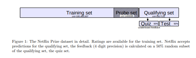
[Image source: Töscher et al. 2009]

Matrix factorization techniques for recommender systems

At the end of the day, the team BellKor’s Pragmatic Chaos, which was a hybrid of two teams KorBell and Big Chaos, won the $1 million grand prize. KorBell, comprising researchers from AT&T, won the first Progress Prize milestone during the early stage of the challenge. Koren et al. (2009) published the article Matrix Factorization Techniques for Recommender Systems in IEEE Computer, summarizing state-of-the-art techniques in matrix factorization and how they can be applied for recommendation tasks in the wild.

However, the BellKor’s Pragmatic Chaos team not only utilizd matrix factorization methods but also blended diverse collaborative filtering algorithms including the Restricted Boltzmann Machine, k-Nearest Neighbors, and MF (Töscher et al. 2009). Furthermore, in fact, MF itself is not a single model, but a loose term to refer to latent models that represent user and items in a low-dimensional latent space. Moreover, with more and more researchers diving into the field, many variants of the initial MF algorithms have been proposed to accomodate for various issues in real-world recommendation tasks. For example, refer to Funk (2006), Koren (2008), and Zhang et al. (2006) for earlier models.

Nonetheless, most MF models and variants have common components, which are decomposing a (user-item interaction) matrix and learning the latent factors to describe users and items. The factors are like dimensions to measure the features of items or proclivity of users. In Figure 2 (Koren et al. 2009) below, the two factors (dimensions) describe masculinity/femininity (geared towards males/females) and seriousness (serious/escapist) of movies. Note that not only items (movies) but also users can be described in terms of combinations of factors based on their preference patterns.

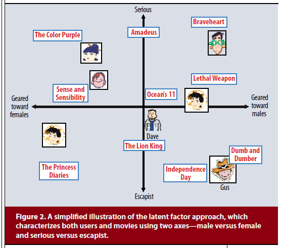
[Image source: Koren et al. 2009]

Nevertheless, individual users’ preference patterns are much more complicated and sometimes inexplicable by nature. For example, Tony loves Mafia movies such as The Godfather, and Scarface, and Donnie Brasco in general. However, he does not like the actor Joe Pesci, making him dislike Mafia movies such as Casino, Goodfellas, and Irishman. In this case, should we encode Tony as liking Mafia movies or not? Should be create another factor having Joe Pesci-ness as a feature?

MF models do most of those dirty jobs for us. They inductively learn the factors and corresponding user/item representations by examining users’ interaction patterns. And this is the most imortant component of most MF algorithms. Various optimization schemes are used for such inference, differentiating many MF models from each other. From the following posting, let’s see how established MF models learn those patterns.

Image source

References

• Gomez-Uribe, C. A., & Hunt, N. (2015). The netflix recommender system: Algorithms, business value, and innovation. ACM Transactions on Management Information Systems (TMIS), 6(4), 1-19.
• Funk, S. (2006) Netflix Update: Try This at Home. (https://sifter.org/~simon/journal/20061211.html)
• Koren, Y., Bell, R., & Volinsky, C. (2009). Matrix factorization techniques for recommender systems. Computer, 42(8), 30-37.
• Koren, Y. (2008, August). Factorization meets the neighborhood: a multifaceted collaborative filtering model. In Proceedings of the 14th ACM SIGKDD international conference on Knowledge discovery and data mining (pp. 426-434).
• Zhang, S., Wang, W., Ford, J., & Makedon, F. (2006, April). Learning from incomplete ratings using non-negative matrix factorization. In Proceedings of the 2006 SIAM international conference on data mining (pp. 549-553). Society for Industrial and Applied Mathematics.
• Töscher, A., Jahrer, M., & Bell, R. M. (2009). The bigchaos solution to the netflix grand prize. Netflix prize documentation, 1-52.
• Ricci, F., Rokach, L., & Shapira, B. (2011). Introduction to recommender systems handbook. In Recommender systems handbook (pp. 1-35). Springer, Boston, MA.

So far, we have covered memory-based collaborative filtering (CF) methods and experimented with the k-Nearest Neighbors (k-NN) algorithm in Python. From now on, let’s switch gears and dig into model-based CF methods.

Model-based CF

We have seen that memory-based CF methods infer ratings based on the memory of previous user-item interaction records. Model-based CF methods are similar in that they make guesses based on previous interaction records. However, instead of relying on pre-computed similarity (or distance) measures, model-based methods employ various prediction models to capture the latent relationship between users and items.

Baseline predictor

In fact, we have already implemented a very simple algorithm for model-based CF, which is the baseline predictor. In general, most recommendation problems show inherent biases, which are overall tendencies that can be generalized on a dataset-level. For instance, some users are generous that they give better ratings than others on average. At the same time, some items have inherently more appealing features than others, resulting in better ratings on average. If you look at the top-100 movies in IMDb, they are rated higher than other movies among the vast majority of users.

Therefore, the baseline estimator tries to guess the magnitude of individual user and item biases. The equation for the estimator is:

\begin{equation} b_{ui} = \mu + b_u + b_i , \end{equation}

where $\mu$ is the average rating across all user-item interactions and $b_u$ and $b_i$ refer to biases for user $u$ and item $i$, respectively. Hence, the baseline predictor tries to quantify how the user and item of interest deviate from the overall average. This is a simple, yet very powerful, idea. In the previous posting, we have seen that it is difficult to beat the baseline predictor with k-NN without incorporating it.

Latent factor models

However, the baseline model has apparent limitations. To start with, it doesn’t consider individual preferences and granular heterogeneity in item features. For instance, Krusty might be a generous and easy-going reviewer in general, but he could be very critical about comedy movies (since he is a clown). Also, Tony could give harsh ratings to most of the movies, but he might have predilections for De Niro movies such as Goodfellas and Irishman (since he is a mafia). Nonetheless, the baseline model aggregates all those information on user- and item-levels, forgoing the granularity.

Therefore, more sophisticated models, namely latent factor models, have been proposed to model complex collaborative patterns. Such patterns are highly non-linear and non-transitive. One of the seminal models have been popularized during the Netflix Prize (Funk 2006), the matrix factorization (MF) model. Recall that memory-based models are good at memorization in general, whereas model-based methods are good at generalization. MF-based models are suited for such generalization tasks.

Do you remember the user-item interaction matrix comprising rating records? MF models attempt to decompose that matrix into two matrices that characterize users and items, respectively. In doing so, the difference between the predicted ratings and actual ratigns are minimized. We will look into MF in detail in the following postings.

[Image source]

Deep recommender systems

MF is a great model with apparent strengths. However, it also has some limitations as recommendation problems gets more complicated. Sometimes, the model architeture is too simple to capture highly complex interaction patterns. Also, it cannot incorporate side information reflecting the context and content. With recent advances in big data, more and more recommendation problems require the prediction model to ingest diverse modes of data such as image and text for optimal performance. Hence, more and more systems adopt deep learning architecture for prediction.

Deep learning provides a great amount of flexibility in terms of model architecture and input data, e.g., neural collaborative filtering (He et al. 2017) and wide & deep learning (Cheng et al. 2016). In the following postings, we will also look at recent developments in deep recommender systems.

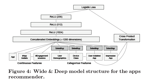
[Image source: Cheng et al. (2016)]

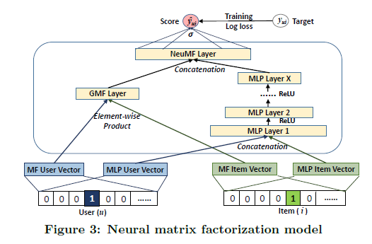
[Image source: He et al. (2017)]

References

• Cheng, H. T., Koc, L., Harmsen, J., Shaked, T., Chandra, T., Aradhye, H., … & Anil, R. (2016, September). Wide & deep learning for recommender systems. In Proceedings of the 1st workshop on deep learning for recommender systems (pp. 7-10).
• Funk, S. (2006) Netflix Update: Try This at Home. (https://sifter.org/~simon/journal/20061211.html)
• He, X., Liao, L., Zhang, H., Nie, L., Hu, X., & Chua, T. S. (2017, April). Neural collaborative filtering. In Proceedings of the 26th international conference on world wide web (pp. 173-182).
• Matrix Factorization (https://developers.google.com/machine-learning/recommendation/collaborative/matrix)
• Koren, Y. (2010). Factor in the neighbors: Scalable and accurate collaborative filtering. ACM Transactions on Knowledge Discovery from Data (TKDD), 4(1), 1-24.
• Ricci, F., Rokach, L., & Shapira, B. (2011). Introduction to recommender systems handbook. In Recommender systems handbook (pp. 1-35). Springer, Boston, MA.