In the previous posting, we have briefly gone through the Netflix Prize, which made Matrix Factorization (MF) methods famous. In this posting, let’s dig into MF methods.

MF as a family of methods

As described earlier, MF for recommendation is a loosely defined term to denote methods that decomposes a rating matrix for collaborative filtering. Hence, it could be regarded as a family of methods involving matrix decomposition procedure. However, methods that are categorized as MF show some common properties. In the remainder of this posting, let’s see what those properties are.

MF basics

User-item interaction matrix revisited

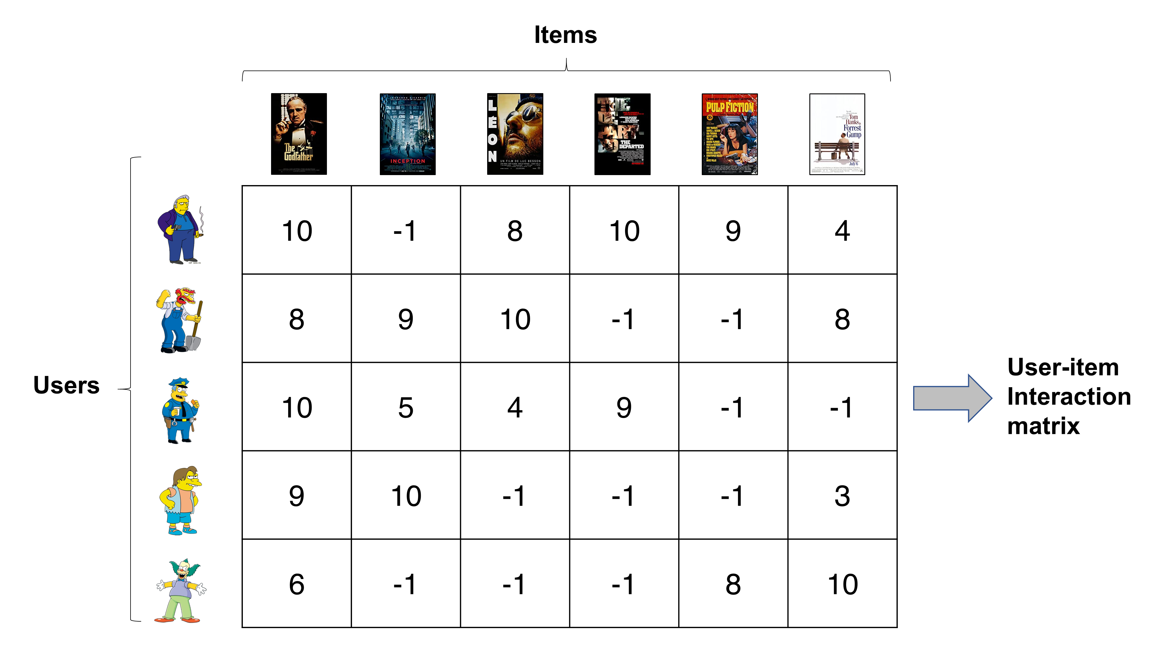
We return to the user-item interaction matrix again. To recap, user-item interaction matrices generally lists users and items in rows and columns, respectively. Then, the interaction records between them are represented as corresponding elements in the matrix. Below matrix is an example of an interaction matrix in a movie recommender engine. Rows in the matrix shows how each user rated items (movies) and columns show how each movie is rated by all users. For more information on user-item interaction matrices, please refer to this posting.

Decomposition of the user-item interaction matrix

After the user-item interaction matrix is generated, it has to be decomposed into two matrices, which are the user matrix ($Q$) and item matrix ($P$). The user and matrices contain descriptions of users and items respectively with learned features. Those features are determined by the developer as they would be in content-based recommender systems. They are intrinsic features of users and items that are unearthed by the algorithm - this is also the reason why MF models are also known as latent factor models.

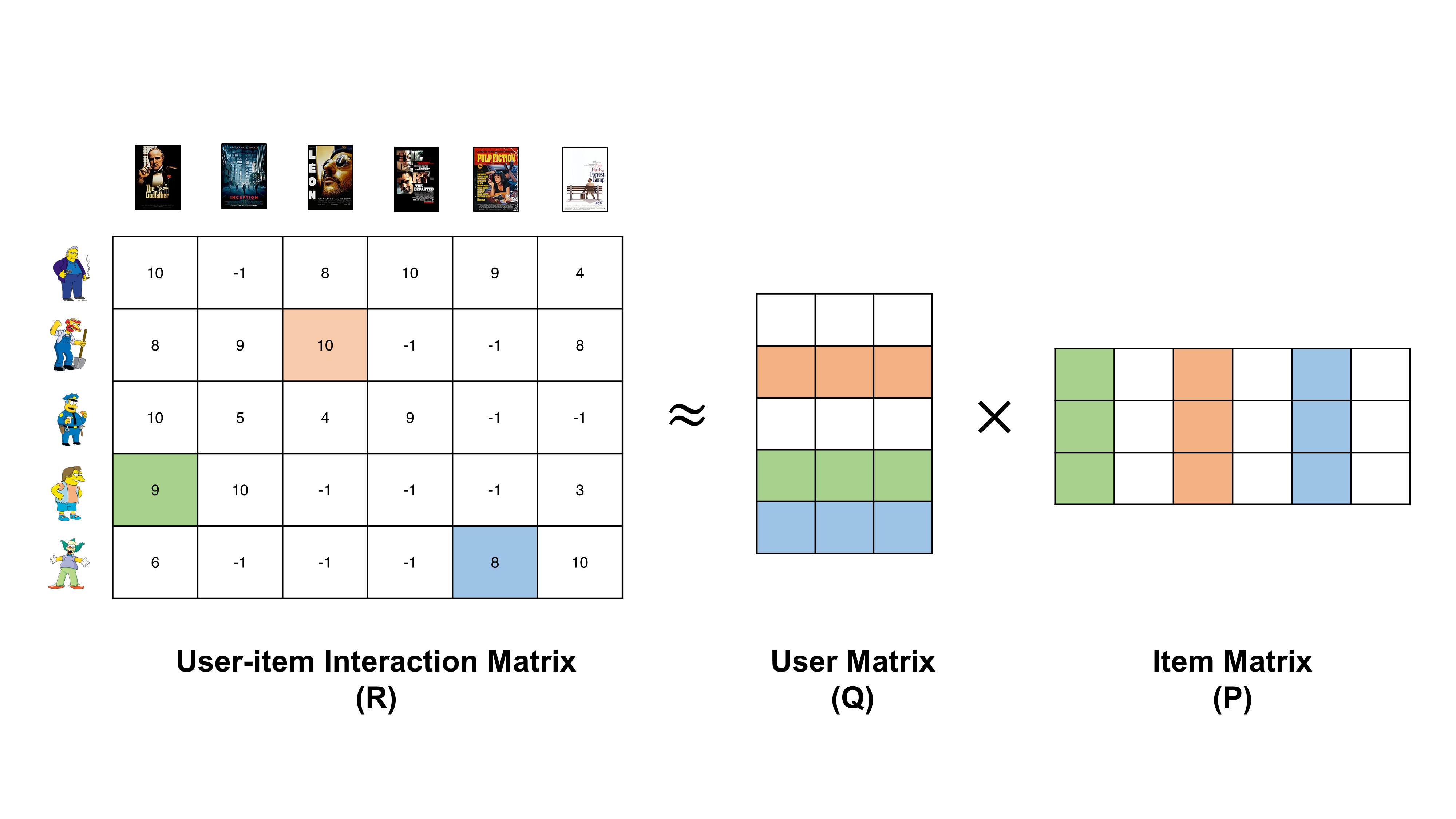
The low-dimensional, latent features are characterized by the algorithm such that they capture correlational patterns in previous user-item interaction records. Therefore, when properly estimated, the user and item matrices can precisely approximate previous user-item interaction patterns and ultimately, used to predict unknown records in the rating matrix. Take the example above of decomposing movie rating matrix. Here, the number of latent features is set to 3 - this is an arbitrary number set by the developer (generally set to a value significantly smaller than the number of users or items). Each row of $Q$ ($q_i$) describes each user and each column of $P$ ($p_j$) describes each movie. And the dot product of $q_i$ and $p_j$ is the estimated rating by the corresponding user to the movie. In a succint equation form,

\begin{equation} r_{ij} = q_{i}p_{j} \end{equation}

The second row of $Q$ represents the second user, i.e., Willie, and the third column of $P$ represents the third item, i.e., Leon. Hence, the dot product of the two results in the estimated rating by Willie to the movie Leon (see orange-colored cells above). Now, can you see how Nelson’s rating on the Godfather and Krusty’s rating on Pulp Fiction can be approximated by elements in $Q$ and $P$? (see green- and blue-colored cells above).

Now, the remaining question is how the algorithm does its magic of decomposing the matrix while considering correlational information? Certainly, putting random numbers in $P$ and $Q$ won’t capture such information. The secret is in the optimization process.

Optimization

The optimization process, like in any other machine learning algorithms, lies at the heart of MF models. And most variants of MF models vary in temrs of how they are optimized when estimating values in user and item matrices. The most simplest way is to minimize the squared differences between the true rating ($r_{ij}$) and estimated rating ($q_{i}p_{j}$) over all $i$ and $j$ that have observed ratings.

\begin{equation} minimize \sum_{i, j} difference(r_{ij} - q_{i}p_{j}) \end{equation}

This is not a bad scheme and do a good job in many cases. However, it does not generalize well in cases where the matrix is binary, i.e., 0 or 1, or skewed. Also, it does not take into account implicit feedback - only explicit feedback is used for optimization. In the following posting, let’s see how different algorithms tried to tackle these problems.

References

• Funk, S. (2006) Netflix Update: Try This at Home. (https://sifter.org/~simon/journal/20061211.html)
• Koren, Y., Bell, R., & Volinsky, C. (2009). Matrix factorization techniques for recommender systems. Computer, 42(8), 30-37.
• Ricci, F., Rokach, L., & Shapira, B. (2011). Introduction to recommender systems handbook. In Recommender systems handbook (pp. 1-35). Springer, Boston, MA.