Buomsoo Kim

Attention in Neural Networks - 21. Transformer (5)

|

Attention Mechanism in Neural Networks - 21. Transformer (5)

In addition to improved performance and alignment between the input and output, attention mechanism provides possible explanations for how the model works. Despite the controversy over the “explainability” of attention mechanisms (e.g., Jain and Wallace, Wiegreffe and Pinter), examining attention weights is one of the few possible ways to understand the inner workings of complex deep neural network systems. However, nn.Transformer does not provide us with innate functionalities to extract and visualize weights. But the good news is that with just a few adjustments and tweaks using the original source code, we can make them fetch the weights and visualize them with matplotlib.

Data import & processing

As we did in the previous posting, let’s import the IMDB movie review sample dataset from the fastai library. But, let’s keep the maximum length of the sequence to 10 for fast and simple implementation.

from fastai.text import *
path = untar_data(URLs.IMDB_SAMPLE)
data = pd.read_csv(path/'texts.csv')
MAX_REVIEW_LEN = 10
reviews, labels = [], []
unique_tokens = set()

for i in tqdm(range(len(data))):
  review = [x.lower() for x in re.findall(r"\w+", data.iloc[i]["text"])]
  if len(review) >= MAX_REVIEW_LEN:
      review = review[:MAX_REVIEW_LEN]
  else:
    for _ in range(MAX_REVIEW_LEN - len(review)):
      review.append("<pad>")

  reviews.append(review)
  unique_tokens.update(review)

  if data.iloc[i]["label"] == 'positive':
    labels.append(1)
  else:
    labels.append(0)

unique_tokens = list(unique_tokens)

# print the size of the vocabulary
print(len(unique_tokens))

# encode each token into index
for i in tqdm(range(len(reviews))):
  reviews[i] = [unique_tokens.index(x) for x in reviews[i]]

Example of processed (and raw) review text.

print(reviews[5])
print([unique_tokens[x] for x in reviews[5]])
[966, 2260, 155, 1439, 254, 2222, 2305, 1257, 1309, 1455] ['un', 'bleeping', 'believable', 'meg', 'ryan', 'doesn', 't', 'even', 'look', 'her']

Setting parameters

Setting parameters is fairly similar to the previous posting. But, since there is no target sequence to predict and we will not make use of the decoder, so parameter settings related to those are unnecessary. Instead, we need an additional hyperparameter of NUM_LABELS that indicates the number of classes in the target variable.

VOCAB_SIZE = len(unique_tokens)
NUM_EPOCHS = 100
HIDDEN_SIZE = 16
EMBEDDING_DIM = 30
BATCH_SIZE = 128
NUM_HEADS = 3
NUM_LAYERS = 3
NUM_LABELS = 2
DROPOUT = .5
LEARNING_RATE = 1e-3
DEVICE = torch.device('cuda') 

Creating dataset & dataloader

We split the dataset to training and test data in 8-2 ratio, resulting in 800 training instances and 200 test instances.

class IMDBDataset(torch.utils.data.Dataset):
  def __init__(self):
    # import and initialize dataset    
    self.x = np.array(reviews, dtype = int)
    self.y = np.array(labels, dtype = int)

  def __getitem__(self, idx):
    # get item by index
    return self.x[idx], self.y[idx]
  
  def __len__(self):
    # returns length of data
    return len(self.x)

np.random.seed(777)   # for reproducibility
dataset = IMDBDataset()
NUM_INSTANCES = len(dataset)
TEST_RATIO = 0.2
TEST_SIZE = int(NUM_INSTANCES * 0.2)

indices = list(range(NUM_INSTANCES))

test_idx = np.random.choice(indices, size = TEST_SIZE, replace = False)
train_idx = list(set(indices) - set(test_idx))
train_sampler, test_sampler = SubsetRandomSampler(train_idx), SubsetRandomSampler(test_idx)

train_loader = torch.utils.data.DataLoader(dataset, batch_size = BATCH_SIZE, sampler = train_sampler)
test_loader = torch.utils.data.DataLoader(dataset, batch_size = BATCH_SIZE, sampler = test_sampler)
torch.Size([128, 10]) torch.Size([128, 10])

Multihead attention

As explained earlier, nn.Transformer makes use of nn.MultiheadAttention module which performs the multihead attention operation given queries, keys, and values. If we closely examine the source code, it has two outputs, i.e., attn_output and attn_output_weights.

- Outputs: - attn_output: :math:`(L, N, E)` where L is the target sequence length, N is the batch size, E is the embedding dimension. - attn_output_weights: :math:`(N, L, S)` where N is the batch size, L is the target sequence length, S is the source sequence length.

So far, we only utilized attn_output that is fed into the final dense layer for classification. We can explicitly observe this from the first line of the forward function TransformerEncoderLayer. (self.self_attn is defined as MultiheadAttention(d_model, nhead, dropout=dropout) in the initialization process).

def forward(self, src, src_mask=None, src_key_padding_mask=None):
  src2 = self.self_attn(src, src, src, attn_mask=src_mask, key_padding_mask= src_key_padding_mask)[0]

So, our strategy will be utilizing attn_output_weights that shows the alignment between the target and source. To do so, we will make use of both inputs from self.self.attn().

Transformer encoder layer

First and foremost, we need to make adjustment to TransformerEncoderLayer. After defining the _get_activation_fn function, add nn. to each module, e.g., MultiheadAttention(d_model, nhead, dropout=dropout) to nn.MultiheadAttention(d_model, nhead, dropout=dropout). And most important, record the alignment weights from self.self_attn, i.e., the multihead attention, and return it with the attention output(src2).

def _get_activation_fn(activation):
    if activation == "relu":
        return F.relu
    elif activation == "gelu":
        return F.gelu

    raise RuntimeError("activation should be relu/gelu, not {}".format(activation))

class TransformerEncoderLayer(Module):
    def __init__(self, d_model, nhead, dim_feedforward=2048, dropout=0.1, activation="relu"):
        super(TransformerEncoderLayer, self).__init__()
        self.self_attn = nn.MultiheadAttention(d_model, nhead, dropout=dropout)
        # Implementation of Feedforward model
        self.linear1 = nn.Linear(d_model, dim_feedforward)
        self.dropout = nn.Dropout(dropout)
        self.linear2 = nn.Linear(dim_feedforward, d_model)

        self.norm1 = nn.LayerNorm(d_model)
        self.norm2 = nn.LayerNorm(d_model)
        self.dropout1 = nn.Dropout(dropout)
        self.dropout2 = nn.Dropout(dropout)

        self.activation = _get_activation_fn(activation)
        
    def __setstate__(self, state):
        if 'activation' not in state:
            state['activation'] = F.relu
        super(TransformerEncoderLayer, self).__setstate__(state)

    def forward(self, src, src_mask=None, src_key_padding_mask=None):
        # type: (Tensor, Optional[Tensor], Optional[Tensor]) -> Tensor
        src2, weights = self.self_attn(src, src, src, attn_mask=src_mask,
                              key_padding_mask=src_key_padding_mask)
        src = src + self.dropout1(src2)
        src = self.norm1(src)
        src2 = self.linear2(self.dropout(self.activation(self.linear1(src))))
        src = src + self.dropout2(src2)
        src = self.norm2(src)
        return src, weights

Transformer encoder

Now we can make adjustments to the transformer encoder. First, define _get_clones function that copies encoder layers. Do not forget to import copy and and nn. to ModuleList. And, similar to what we did before, we need to record the calculated alignment weights. Let’s explicitly make a list weights to save the weight from each layer. Again, this layer has to be returned with the final attention output.

import copy

def _get_clones(module, N):
    return nn.ModuleList([copy.deepcopy(module) for i in range(N)])

class TransformerEncoder(Module):
    __constants__ = ['norm']
    def __init__(self, encoder_layer, num_layers, norm=None):
        super(TransformerEncoder, self).__init__()
        self.layers = _get_clones(encoder_layer, num_layers)
        self.num_layers = num_layers
        self.norm = norm

    def forward(self, src, mask=None, src_key_padding_mask=None):
        # type: (Tensor, Optional[Tensor], Optional[Tensor]) -> Tensor
        output = src
        weights = []
        for mod in self.layers:
            output, weight = mod(output, src_mask=mask, src_key_padding_mask=src_key_padding_mask)
            weights.append(weight)

        if self.norm is not None:
            output = self.norm(output)
        return output, weights

Transformer

Finally, we can define the entire Transformer architecture with the building blocks. The process of fetching and returning both weights and outputs is similar to what we did with RNN Encoder-Decoders.

class TransformerNet(nn.Module):
    def __init__(self, num_vocab, embedding_dim, hidden_size, nheads, n_layers, max_len, num_labels, dropout):
        super(TransformerNet, self).__init__()
        # embedding layer
        self.embedding = nn.Embedding(num_vocab, embedding_dim)
        # positional encoding layer
        self.pe = PositionalEncoding(embedding_dim, max_len = max_len)
        # encoder  layers
        enc_layer = TransformerEncoderLayer(embedding_dim, nheads, hidden_size, dropout)
        self.encoder = TransformerEncoder(enc_layer, num_layers = n_layers)
        # final dense layer
        self.dense = nn.Linear(embedding_dim*max_len, num_labels)
        self.log_softmax = nn.LogSoftmax()

    def forward(self, x):
        x = self.embedding(x).permute(1, 0, 2)
        x = self.pe(x)
        x, w = self.encoder(x)
        x = x.reshape(x.shape[1], -1)
        x = self.dense(x)
        return x, w
model = TransformerNet(VOCAB_SIZE, EMBEDDING_DIM, HIDDEN_SIZE, NUM_HEADS, NUM_LAYERS, MAX_REVIEW_LEN, NUM_LABELS, DROPOUT).to(DEVICE)
criterion = nn.CrossEntropyLoss()
optimizer = torch.optim.Adam(model.parameters(), lr = LEARNING_RATE)

Training

Training is also straightforward, just be aware of recording the weights (w) from the model.

%%time
loss_trace = []
for epoch in tqdm(range(NUM_EPOCHS)):
  current_loss = 0
  for i, (x, y) in enumerate(train_loader):
    x, y  = x.to(DEVICE), y.to(DEVICE)
    outputs, w = model(x)
    loss = criterion(outputs, y)
    optimizer.zero_grad()
    loss.backward()
    optimizer.step()
    current_loss += loss.item()
  loss_trace.append(current_loss)

Visualization

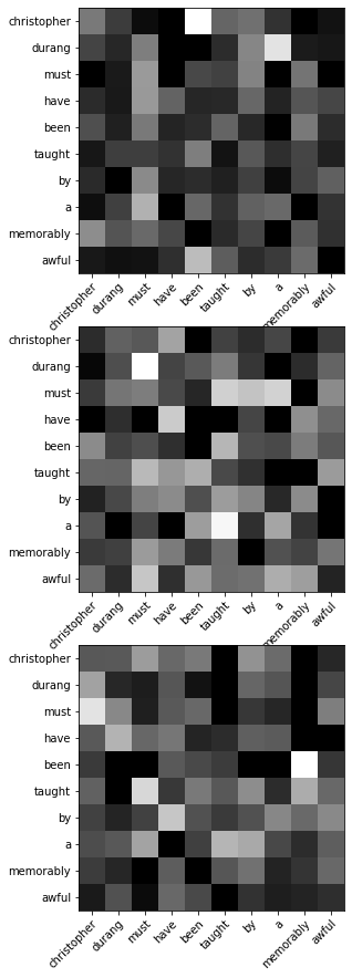
Let’s try visualizing the alignment weights for the last training instance. w list has three tensors as elements, each as outputs from each encoder layer. Each tensor has the shape of (N, S, S), or (batch size, source sequence length, source sequence length).

print(len(w))
print(w[0].shape)
3 torch.Size([32, 10, 10])
input_sentence = x[-1].detach().cpu().numpy()
input_sentence = [unique_tokens[x] for x in input_sentence]

fig, axes = plt.subplots(nrows = 3, ncols = 1, figsize = (5, 15), facecolor = "w")
for i in range(len(w)):
  axes[i].imshow(w[i][-1].detach().cpu().numpy(), cmap = "gray")
  axes[i].set_yticks(np.arange(len(input_sentence)))
  axes[i].set_yticklabels(input_sentence)
  axes[i].set_xticks(np.arange(len(input_sentence)))
  axes[i].set_xticklabels(input_sentence)
  plt.setp(axes[i].get_xticklabels(), rotation=45, ha="right",
         rotation_mode="anchor")
plt.show()
References

Attention in Neural Networks - 20. Transformer (4)

|

Attention Mechanism in Neural Networks - 20. Transformer (4)

So far, we have seen how the Transformer architecture can be used for the machine translation task. However, Transformer and more generally, self-attention can be used for other prediction tasks as well. Here, let’s see how we can exploit the Transformer architecture for sentence classification task. We created a sentence classification model with the Hierarchical Attention Networks (HAN) architecture in one of previous postings. The model in this posting will be similar, but without the hierarchical attention and RNNs.

Data import

For simplicity, let’s import the IMDB movie review sample dataset from the fastai library. By the way, fastai provides many convenient and awesome functionalities for not just data import/processing but also quick and easy implementation, training, evaluation, and visualization. They also offer free lecture videos and tutorials that you can check out here.

from fastai.text import *
path = untar_data(URLs.IMDB_SAMPLE)
data = pd.read_csv(path/'texts.csv')
data.head()
label text is_valid 0 negative Un-bleeping-believable! Meg Ryan doesn't even ... False 1 positive This is a extremely well-made film. The acting... False 2 negative Every once in a long while a movie will come a... False 3 positive Name just says it all. I watched this movie wi... False 4 negative This movie succeeds at being one of the most u... False

Data Preprocessing

Now, we have to process the data as we did for HAN. However, here we do not need to consider the hierarchical structure of sentences and words, so it is much simpler. There are 1,000 movie reviews and 5,317 unique tokens when setting the maximum length of review (MAX_REVIEW_LEN) to 20.

MAX_REVIEW_LEN = 20
reviews, labels = [], []
unique_tokens = set()

for i in tqdm(range(len(data))):
  review = [x.lower() for x in re.findall(r"\w+", data.iloc[i]["text"])]
  if len(review) >= MAX_REVIEW_LEN:
      review = review[:MAX_REVIEW_LEN]
  else:
    for _ in range(MAX_REVIEW_LEN - len(review)):
      review.append("<pad>")

  reviews.append(review)
  unique_tokens.update(review)

  if data.iloc[i]["label"] == 'positive':
    labels.append(1)
  else:
    labels.append(0)

unique_tokens = list(unique_tokens)

# print the size of the vocabulary
print(len(unique_tokens))

# encode each token into index
for i in tqdm(range(len(reviews))):
  reviews[i] = [unique_tokens.index(x) for x in reviews[i]]

Example of processed (and raw) review text.

print(reviews[0])
print([unique_tokens[x] for x in reviews[0]])
[663, 2188, 53, 3336, 1155, 325, 176, 1727, 1666, 1934, 283, 2495, 105, 130, 2498, 1979, 2598, 3056, 2981, 2424] ['un', 'bleeping', 'believable', 'meg', 'ryan', 'doesn', 't', 'even', 'look', 'her', 'usual', 'pert', 'lovable', 'self', 'in', 'this', 'which', 'normally', 'makes', 'me']

Setting parameters

Setting parameters is fairly similar to the previous posting. But, since there is no target sequence to predict and we will not make use of the decoder, so parameter settings related to those are unnecessary. Instead, we need an additional hyperparameter of NUM_LABELS that indicates the number of classes in the target variable.

VOCAB_SIZE = len(unique_tokens)
NUM_EPOCHS = 100
HIDDEN_SIZE = 16
EMBEDDING_DIM = 30
BATCH_SIZE = 128
NUM_HEADS = 3
NUM_LAYERS = 3
NUM_LABELS = 2
DROPOUT = .5
LEARNING_RATE = 1e-3
DEVICE = torch.device('cuda') 

Creating dataset & dataloader

We split the dataset to training and test data in 8-2 ratio, resulting in 800 training instances and 200 test instances.

class IMDBDataset(torch.utils.data.Dataset):
  def __init__(self):
    # import and initialize dataset    
    self.x = np.array(reviews, dtype = int)
    self.y = np.array(labels, dtype = int)

  def __getitem__(self, idx):
    # get item by index
    return self.x[idx], self.y[idx]
  
  def __len__(self):
    # returns length of data
    return len(self.x)

np.random.seed(777)   # for reproducibility
dataset = IMDBDataset()
NUM_INSTANCES = len(dataset)
TEST_RATIO = 0.2
TEST_SIZE = int(NUM_INSTANCES * 0.2)

indices = list(range(NUM_INSTANCES))

test_idx = np.random.choice(indices, size = TEST_SIZE, replace = False)
train_idx = list(set(indices) - set(test_idx))
train_sampler, test_sampler = SubsetRandomSampler(train_idx), SubsetRandomSampler(test_idx)

train_loader = torch.utils.data.DataLoader(dataset, batch_size = BATCH_SIZE, sampler = train_sampler)
test_loader = torch.utils.data.DataLoader(dataset, batch_size = BATCH_SIZE, sampler = test_sampler)
torch.Size([128, 10]) torch.Size([128, 10])

Transformer network for text classification

As mentioned, we do not need a decoder since we do not have additional sequences to predict. Instead, the outputs from encoder layers are directly passed on to the final dense layer. Therefore, the model structure is much simpler, but be aware of the tensor shapes. The output tensor from the encoder has to be reshaped to match the target.

## source: https://pytorch.org/tutorials/beginner/transformer_tutorial.html
class PositionalEncoding(nn.Module):
    def __init__(self, d_model, dropout=0.1, max_len=5000):
        super(PositionalEncoding, self).__init__()
        self.dropout = nn.Dropout(p=dropout)
        pe = torch.zeros(max_len, d_model)
        position = torch.arange(0, max_len, dtype=torch.float).unsqueeze(1)
        div_term = torch.exp(torch.arange(0, d_model, 2).float() * (-np.log(10000.0) / d_model))
        pe[:, 0::2] = torch.sin(position * div_term)
        pe[:, 1::2] = torch.cos(position * div_term)
        pe = pe.unsqueeze(0).transpose(0, 1)
        self.register_buffer('pe', pe)

    def forward(self, x):
        x = x + self.pe[:x.size(0), :]
        return self.dropout(x)

class TransformerNet(nn.Module):
  def __init__(self, num_vocab, embedding_dim, hidden_size, nheads, n_layers, max_len, num_labels, dropout):
    super(TransformerNet, self).__init__()
    # embedding layer
    self.embedding = nn.Embedding(num_vocab, embedding_dim)
    
    # positional encoding layer
    self.pe = PositionalEncoding(embedding_dim, max_len = max_len)

    # encoder  layers
    enc_layer = nn.TransformerEncoderLayer(embedding_dim, nheads, hidden_size, dropout)
    self.encoder = nn.TransformerEncoder(enc_layer, num_layers = n_layers)

    # final dense layer
    self.dense = nn.Linear(embedding_dim*max_len, num_labels)
    self.log_softmax = nn.LogSoftmax()

  def forward(self, x):
    x = self.embedding(x).permute(1, 0, 2)
    x = self.pe(x)
    x = self.encoder(x)
    x = x.reshape(x.shape[1], -1)
    x = self.dense(x)
    return x
    
model = TransformerNet(VOCAB_SIZE, EMBEDDING_DIM, HIDDEN_SIZE, NUM_HEADS, NUM_LAYERS, MAX_REVIEW_LEN, NUM_LABELS, DROPOUT).to(DEVICE)
criterion = nn.CrossEntropyLoss()
optimizer = torch.optim.Adam(model.parameters(), lr = LEARNING_RATE)

Training

Training process is largely similar. Again, we just need to be mindful of the output and corresponding target tensor shapes.

%%time
loss_trace = []
for epoch in tqdm(range(NUM_EPOCHS)):
  current_loss = 0
  for i, (x, y) in enumerate(train_loader):
    x, y  = x.to(DEVICE), y.to(DEVICE)
    outputs = model(x)
    loss = criterion(outputs, y)
    optimizer.zero_grad()
    loss.backward()
    optimizer.step()
    current_loss += loss.item()
  loss_trace.append(current_loss)

# loss curve
plt.plot(range(1, NUM_EPOCHS+1), loss_trace, 'r-')
plt.xlabel('Epoch')
plt.ylabel('Loss')
plt.show()

Evaluation

Finally, we can evaluate the model by comparing the output and test target data. From my trained model, the result is not that satisfactory with accuracy around 50%. There can be many reasons for this, such as insufficient hyperparameter tuning and data quality issues. Therefore, for optimal performances, I recommend trying many different architectures and settings to find out the most suitable model for your dataset and task!

correct, total = 0, 0
predictions = []
for i, (x,y) in enumerate(test_loader):
  with torch.no_grad():
    x, y  = x.to(DEVICE), y.to(DEVICE)
    outputs = model(x)
    _, y_pred = torch.max(outputs.data, 1)
    total += y.shape[0]
    correct += (y_pred == y).sum().item()

print(correct/total)
0.495

References

Attention in Neural Networks - 19. Transformer (3)

|

Attention Mechanism in Neural Networks - 19. Transformer (3)

In the previous posting, we tried implementing the simple Transformer architecture with nn.Transformer. In this posting, let’s dig a little deeper and see how nn.Transformer works under the hood.

Data import & preprocessing

Steps up to creating dataset and datalodaer are almost identical. So you can skim through these preliminary steps if you are familar with.

Using Jupyter Notebook or Google Colaboratory, the data file can be fetched directly from the Web and unzipped.

!wget https://www.manythings.org/anki/deu-eng.zip
!unzip deu-eng.zip

with open("deu.txt") as f:
  sentences = f.readlines()

As we did before, let’s randomly sample 10,000 instances and process them.

NUM_INSTANCES = 10000
MAX_SENT_LEN = 10
eng_sentences, deu_sentences = [], []
eng_words, deu_words = set(), set()
for i in tqdm(range(NUM_INSTANCES)):
  rand_idx = np.random.randint(len(sentences))
  # find only letters in sentences
  eng_sent, deu_sent = ["<sos>"], ["<sos>"]
  eng_sent += re.findall(r"\w+", sentences[rand_idx].split("\t")[0]) 
  deu_sent += re.findall(r"\w+", sentences[rand_idx].split("\t")[1])

  # change to lowercase
  eng_sent = [x.lower() for x in eng_sent]
  deu_sent = [x.lower() for x in deu_sent]
  eng_sent.append("<eos>")
  deu_sent.append("<eos>")

  if len(eng_sent) >= MAX_SENT_LEN:
    eng_sent = eng_sent[:MAX_SENT_LEN]
  else:
    for _ in range(MAX_SENT_LEN - len(eng_sent)):
      eng_sent.append("<pad>")

  if len(deu_sent) >= MAX_SENT_LEN:
    deu_sent = deu_sent[:MAX_SENT_LEN]
  else:
    for _ in range(MAX_SENT_LEN - len(deu_sent)):
      deu_sent.append("<pad>")

  # add parsed sentences
  eng_sentences.append(eng_sent)
  deu_sentences.append(deu_sent)

  # update unique words
  eng_words.update(eng_sent)
  deu_words.update(deu_sent)

eng_words, deu_words = list(eng_words), list(deu_words)

# encode each token into index
for i in tqdm(range(len(eng_sentences))):
  eng_sentences[i] = [eng_words.index(x) for x in eng_sentences[i]]
  deu_sentences[i] = [deu_words.index(x) for x in deu_sentences[i]]

idx = 10
print(eng_sentences[idx])
print([eng_words[x] for x in eng_sentences[idx]])
print(deu_sentences[idx])
print([deu_words[x] for x in deu_sentences[idx]])

If properly imported and processed, you will get an output something like this. But specific values of output will be somewhat different since we are randomly sampling instances.

[2142, 1843, 174, 3029, 1716, 3449, 4385, 2021, 4359, 4359]
['<sos>', 'tom', 'didn', 't', 'have', 'a', 'chance', '<eos>', '<pad>', '<pad>']
[2570, 6013, 2486, 2470, 1631, 2524, 3415, 3415, 3415, 3415]
['<sos>', 'tom', 'hatte', 'keine', 'chance', '<eos>', '<pad>', '<pad>', '<pad>', '<pad>']

Setting Parameters

Most of paramter setting is similar to the RNN Encoder-Decoder network and its variants.

  • HIDDEN SIZE: previously this was used to set the number of hidden cells in the RNN network. However, here it will be used to set the dimensionality of the feedforward network, or the dense layers.
  • NUM_LAYERS: similary, instead of setting the number of RNN layers, this is used to determine the number of dense layers.
  • NUM_HEADS: this is a new parameter used to determine the number of heads in multihead attention. If you are unsure what multihead attention is, refer to the previous posting.
  • DROPOUT: Another parameter that we can consider is DROPOUT, which determines the probability of dropping out a node in the encoder/decoder layer. This can be set to the same value across all layers, or can be fine-tuned to set to different values in each layer. However, in most cases it is a single value across all layers for simplicity.
ENG_VOCAB_SIZE = len(eng_words)
DEU_VOCAB_SIZE = len(deu_words)
NUM_EPOCHS = 10
HIDDEN_SIZE = 16
EMBEDDING_DIM = 30
BATCH_SIZE = 128
NUM_HEADS = 2
NUM_LAYERS = 3
LEARNING_RATE = 1e-2
DROPOUT = .3
DEVICE = torch.device('cuda') 

Creating dataset and dataloader

This is exactly the same step as before, so I won’t explain the details. Again, if you want to know more, please refer to the previous postings.

class MTDataset(torch.utils.data.Dataset):
  def __init__(self):
    # import and initialize dataset    
    self.source = np.array(eng_sentences, dtype = int)
    self.target = np.array(deu_sentences, dtype = int)
    
  def __getitem__(self, idx):
    # get item by index
    return self.source[idx], self.target[idx]
  
  def __len__(self):
    # returns length of data
    return len(self.source)

np.random.seed(777)   # for reproducibility
dataset = MTDataset()
NUM_INSTANCES = len(dataset)
TEST_RATIO = 0.3
TEST_SIZE = int(NUM_INSTANCES * 0.3)

indices = list(range(NUM_INSTANCES))

test_idx = np.random.choice(indices, size = TEST_SIZE, replace = False)
train_idx = list(set(indices) - set(test_idx))
train_sampler, test_sampler = SubsetRandomSampler(train_idx), SubsetRandomSampler(test_idx)

train_loader = torch.utils.data.DataLoader(dataset, batch_size = BATCH_SIZE, sampler = train_sampler)
test_loader = torch.utils.data.DataLoader(dataset, batch_size = BATCH_SIZE, sampler = test_sampler)

Under the hood of nn.Transformer

The best way to understand how Pytorch models work is by analyzing tensor operations between layers and functions. In most cases, we do not need to attend to the specific values of tensors, but just can keep track of tensor shapes, or sizes. Making sense of how each element in the size (shape) array is mapped to dimensionality of input/output tensors and how they are manipulated with matrix operations are critical.

Here, let’s fetch the first batch of the training data and see how it is transformed step-by-step in the Transformer network.

Each batch tensor from the train_loader has the shape of (BATCH_SIZE, MAX_SENT_LEN).

src, tgt = next(iter(train_loader))
print(src.shape, tgt.shape)   # (BATCH_SIZE, SEQ_LEN)
torch.Size([128, 10]) torch.Size([128, 10])

Embedding

After being embedded, they have the shape of (BATCH_SIZE, MAX_SENT_LEN, EMBEDDING_DIM).

enc_embedding = nn.Embedding(ENG_VOCAB_SIZE, EMBEDDING_DIM)
dec_embedding = nn.Embedding(DEU_VOCAB_SIZE, EMBEDDING_DIM)
src, tgt = enc_embedding(src), dec_embedding(tgt)
print(src.shape, tgt.shape)                # (BATCH_SIZE, SEQ_LEN, EMBEDDING_DIM)
torch.Size([128, 10, 30]) torch.Size([128, 10, 30])

Positional encoding

Then, the embedded tensors have to be positionally encoded to take into account the order of sequences. I borrowed this code from the official Pytorch Tranformer tutorial, after just replacing math.log() with np.log().

## source: https://pytorch.org/tutorials/beginner/transformer_tutorial.html
class PositionalEncoding(nn.Module):
    def __init__(self, d_model, dropout=0.1, max_len=5000):
        super(PositionalEncoding, self).__init__()
        self.dropout = nn.Dropout(p=dropout)
        pe = torch.zeros(max_len, d_model)
        position = torch.arange(0, max_len, dtype=torch.float).unsqueeze(1)
        div_term = torch.exp(torch.arange(0, d_model, 2).float() * (-np.log(10000.0) / d_model))
        pe[:, 0::2] = torch.sin(position * div_term)
        pe[:, 1::2] = torch.cos(position * div_term)
        pe = pe.unsqueeze(0).transpose(0, 1)
        self.register_buffer('pe', pe)

    def forward(self, x):
        x = x + self.pe[:x.size(0), :]
        return self.dropout(x)

Before positional encoding, we swap the first and second dimensions. This can be sometimes unnecessary if your data shape is different or employing different code for positional encoding. And after positional encoding, the tensors have the same shape. Remember that positional encoding is simply element-wise adding information regarding the relative/absolute position without altering the tensor shape.

pe = PositionalEncoding(EMBEDDING_DIM, max_len = MAX_SENT_LEN)
src, tgt = pe(src.permute(1, 0, 2)), pe(tgt.permute(1, 0, 2))
print(src.shape, tgt.shape)              # (SEQ_LEN, BATCH_SIZE, EMBEDDING_DIM)
torch.Size([10, 128, 30]) torch.Size([10, 128, 30])

Encoder

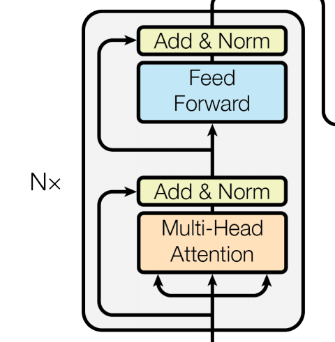
[Image source: Vaswani et al. (2017)]
Now we can pass on the input to the encoder. There are two modules related to the encoder - nn.TransformerEncoderLayer and nn.TransformerEncoder. Remember that the encoder is a stack of $N$ identical layers ($N = 6$ in the Vaswani et al. paper). Each “layer” consists of multi-head attention and position-wise feed-forward networks.

nn.TransformerEncoderLayer generates a single layer and nn.TransformerEncoder basically stacks up $N$ copies of that instance. The output shapes from all layers are identical, making this much simple. Also note that we can specify the dropout rate with the dropout parameter, making nodes in each layer “dropped out” to prevent overfitting.

enc_layer = nn.TransformerEncoderLayer(EMBEDDING_DIM, NUM_HEADS, HIDDEN_SIZE, DROPOUT)
memory = enc_layer(src)
print(memory.shape)                      # (SEQ_LEN, BATCH_SIZE, EMBEDDING_DIM)
torch.Size([10, 128, 30])

nn.TransformerEncoder stacks up NUM_LAYERS copies of encoder layers. The outputs from the encoder are named “memory,” indicating that the encoder memorizes information from source sequences and passes them on to the decoder.

encoder = nn.TransformerEncoder(enc_layer, num_layers = NUM_LAYERS)
memory = encoder(src)
print(memory.shape)                     # (SEQ_LEN, BATCH_SIZE, EMBEDDING_DIM)
torch.Size([10, 128, 30])

Decoder

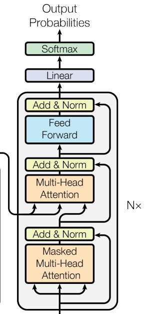
[Image source: Vaswani et al. (2017)]

The decoder architecture is similar, but it has two multi-head attention networks to (1) process the “memory” from the encoder and (2) extract information from target sequences. Therefore, nn.TransformerDecoderLayer and nn.TransformerDecoder have two inputs, tgt and memory.

dec_layer = nn.TransformerDecoderLayer(EMBEDDING_DIM, NUM_HEADS, HIDDEN_SIZE, DROPOUT)
decoder = nn.TransformerDecoder(dec_layer, num_layers = NUM_LAYERS)
transformer_output = decoder(tgt, memory)
print(transformer_output.shape)        # (SEQ_LEN, BATCH_SIZE, EMBEDDING_DIM)
torch.Size([10, 128, 30])

Final dense layer

To classify each token, we need to have an additional layer to calculate the probabilities. The output size of the final dense layer is equivalent to the vocabulary size of target language.

dense = nn.Linear(EMBEDDING_DIM, DEU_VOCAB_SIZE)
final_output = dense(transformer_output)
print(final_output.shape)             # (SEQ_LEN, BATCH_SIZE, EMBEDDING_DIM)
torch.Size([10, 128, 6893])

Putting it together

Now, we can just put all things together and create a blueprint for the Transformer network that can be used for most of sequence-to-sequence mapping tasks.

class TransformerNet(nn.Module):
  def __init__(self, num_src_vocab, num_tgt_vocab, embedding_dim, hidden_size, nheads, n_layers, max_src_len, max_tgt_len, dropout):
    super(TransformerNet, self).__init__()
    # embedding layers
    self.enc_embedding = nn.Embedding(num_src_vocab, embedding_dim)
    self.dec_embedding = nn.Embedding(num_tgt_vocab, embedding_dim)

    # positional encoding layers
    self.enc_pe = PositionalEncoding(embedding_dim, max_len = max_src_len)
    self.dec_pe = PositionalEncoding(embedding_dim, max_len = max_tgt_len)

    # encoder/decoder layers
    enc_layer = nn.TransformerEncoderLayer(embedding_dim, nheads, hidden_size, dropout)
    dec_layer = nn.TransformerDecoderLayer(embedding_dim, nheads, hidden_size, dropout)
    self.encoder = nn.TransformerEncoder(enc_layer, num_layers = n_layers)
    self.decoder = nn.TransformerDecoder(dec_layer, num_layers = n_layers)

    # final dense layer
    self.dense = nn.Linear(embedding_dim, num_tgt_vocab)
    self.log_softmax = nn.LogSoftmax()

  def forward(self, src, tgt):
    src, tgt = self.enc_embedding(src).permute(1, 0, 2), self.dec_embedding(tgt).permute(1, 0, 2)
    src, tgt = self.enc_pe(src), self.dec_pe(tgt)
    memory = self.encoder(src)
    transformer_out = self.decoder(tgt, memory)
    final_out = self.dense(transformer_out)
    return self.log_softmax(final_out)
model = TransformerNet(ENG_VOCAB_SIZE, DEU_VOCAB_SIZE, EMBEDDING_DIM, HIDDEN_SIZE, NUM_HEADS, NUM_LAYERS, MAX_SENT_LEN, MAX_SENT_LEN, DROPOUT).to(DEVICE)
criterion = nn.NLLLoss()
optimizer = torch.optim.Adam(model.parameters(), lr = LEARNING_RATE)

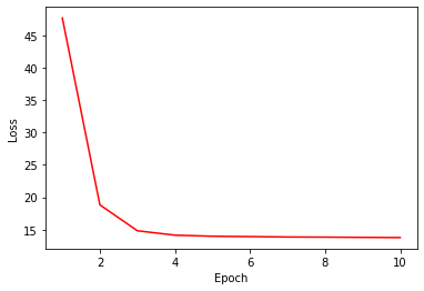
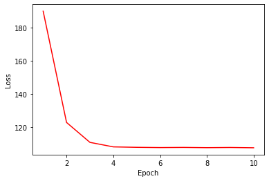
After training, you can see that this Transformer network shows more stable and robust result compared to the one we trained in the previous posting.

%%time
loss_trace = []
for epoch in tqdm(range(NUM_EPOCHS)):
  current_loss = 0
  for i, (x, y) in enumerate(train_loader):
    x, y  = x.to(DEVICE), y.to(DEVICE)
    outputs = model(x, y)
    loss = criterion(outputs.permute(1, 2, 0), y)
    optimizer.zero_grad()
    loss.backward()
    optimizer.step()
    current_loss += loss.item()
  loss_trace.append(current_loss)

# loss curve
plt.plot(range(1, NUM_EPOCHS+1), loss_trace, 'r-')
plt.xlabel('Epoch')
plt.ylabel('Loss')
plt.show()

References

Attention in Neural Networks - 18. Transformer (2)

|

Attention Mechanism in Neural Networks - 18. Transformer (2)

In the previous posting, we have gone through the details of the Transformer architecture proposed by Vaswani et al. (2017). From now on, let’s see how we can implement the Transformer network in Pytorch, using nn.Transformer. The details of Transformer can be very complicated and daunting. However, with some background knowledge obtained from the previous posting and nn.Transformer’s help, it is not so difficult.

Data import & preprocessing

We come back to the English-German machine translation dataset from manythings.org. If you are new here and interested in details, please refer to my previous postings on Seq2Seq.

Using Jupyter Notebook or Google Colaboratory, the data file can be fetched directly from the Web and unzipped.

!wget https://www.manythings.org/anki/deu-eng.zip
!unzip deu-eng.zip

with open("deu.txt") as f:
  sentences = f.readlines()

As we did before, let’s randomly sample 10,000 instances and process them.

NUM_INSTANCES = 10000
MAX_SENT_LEN = 10
eng_sentences, deu_sentences = [], []
eng_words, deu_words = set(), set()
for i in tqdm(range(NUM_INSTANCES)):
  rand_idx = np.random.randint(len(sentences))
  # find only letters in sentences
  eng_sent, deu_sent = ["<sos>"], ["<sos>"]
  eng_sent += re.findall(r"\w+", sentences[rand_idx].split("\t")[0]) 
  deu_sent += re.findall(r"\w+", sentences[rand_idx].split("\t")[1])

  # change to lowercase
  eng_sent = [x.lower() for x in eng_sent]
  deu_sent = [x.lower() for x in deu_sent]
  eng_sent.append("<eos>")
  deu_sent.append("<eos>")

  if len(eng_sent) >= MAX_SENT_LEN:
    eng_sent = eng_sent[:MAX_SENT_LEN]
  else:
    for _ in range(MAX_SENT_LEN - len(eng_sent)):
      eng_sent.append("<pad>")

  if len(deu_sent) >= MAX_SENT_LEN:
    deu_sent = deu_sent[:MAX_SENT_LEN]
  else:
    for _ in range(MAX_SENT_LEN - len(deu_sent)):
      deu_sent.append("<pad>")

  # add parsed sentences
  eng_sentences.append(eng_sent)
  deu_sentences.append(deu_sent)

  # update unique words
  eng_words.update(eng_sent)
  deu_words.update(deu_sent)

eng_words, deu_words = list(eng_words), list(deu_words)

# encode each token into index
for i in tqdm(range(len(eng_sentences))):
  eng_sentences[i] = [eng_words.index(x) for x in eng_sentences[i]]
  deu_sentences[i] = [deu_words.index(x) for x in deu_sentences[i]]

idx = 10
print(eng_sentences[idx])
print([eng_words[x] for x in eng_sentences[idx]])
print(deu_sentences[idx])
print([deu_words[x] for x in deu_sentences[idx]])

If properly imported and processed, you will get an output something like this. But specific values of output will be somewhat different since we are randomly sampling instances.

[2142, 1843, 174, 3029, 1716, 3449, 4385, 2021, 4359, 4359]
['<sos>', 'tom', 'didn', 't', 'have', 'a', 'chance', '<eos>', '<pad>', '<pad>']
[2570, 6013, 2486, 2470, 1631, 2524, 3415, 3415, 3415, 3415]
['<sos>', 'tom', 'hatte', 'keine', 'chance', '<eos>', '<pad>', '<pad>', '<pad>', '<pad>']

Setting Parameters

Most of paramter setting is similar to the RNN Encoder-Decoder network and its variants.

  • HIDDEN SIZE: previously this was used to set the number of hidden cells in the RNN network. However, here it will be used to set the dimensionality of the feedforward network, or the dense layers.
  • NUM_LAYERS: similary, instead of setting the number of RNN layers, this is used to determine the number of dense layers.
  • NUM_HEADS: this is a new parameter used to determine the number of heads in multihead attention. If you are unsure what multihead attention is, refer to the previous posting.
ENG_VOCAB_SIZE = len(eng_words)
DEU_VOCAB_SIZE = len(deu_words)
NUM_EPOCHS = 10
HIDDEN_SIZE = 16
EMBEDDING_DIM = 30
BATCH_SIZE = 128
NUM_HEADS = 2
NUM_LAYERS = 3
LEARNING_RATE = 1e-2
DEVICE = torch.device('cuda') 

Creating dataset and dataloader

This is exactly the same step as before, so I won’t explain the details. Again, if you want to know more, please refer to the previous postings.

class MTDataset(torch.utils.data.Dataset):
  def __init__(self):
    # import and initialize dataset    
    self.source = np.array(eng_sentences, dtype = int)
    self.target = np.array(deu_sentences, dtype = int)
    
  def __getitem__(self, idx):
    # get item by index
    return self.source[idx], self.target[idx]
  
  def __len__(self):
    # returns length of data
    return len(self.source)

np.random.seed(777)   # for reproducibility
dataset = MTDataset()
NUM_INSTANCES = len(dataset)
TEST_RATIO = 0.3
TEST_SIZE = int(NUM_INSTANCES * 0.3)

indices = list(range(NUM_INSTANCES))

test_idx = np.random.choice(indices, size = TEST_SIZE, replace = False)
train_idx = list(set(indices) - set(test_idx))
train_sampler, test_sampler = SubsetRandomSampler(train_idx), SubsetRandomSampler(test_idx)

train_loader = torch.utils.data.DataLoader(dataset, batch_size = BATCH_SIZE, sampler = train_sampler)
test_loader = torch.utils.data.DataLoader(dataset, batch_size = BATCH_SIZE, sampler = test_sampler)

Transformer network in (almost) 10 lines of code

As mentioned, implementing a Transformer network is simple and straightforward. With around 10 lines of code, a simple and straightfoward Transformer network for sequence-to-sequence modeling can be created.

class TransformerNet(nn.Module):
  def __init__(self, num_src_vocab, num_tgt_vocab, embedding_dim, hidden_size, nhead, n_layers):
    super(TransformerNet, self).__init__()
    self.enc_embedding = nn.Embedding(num_src_vocab, embedding_dim)
    self.dec_embedding = nn.Embedding(num_tgt_vocab, embedding_dim)
    self.transformer = nn.Transformer(d_model = embedding_dim, nhead = nhead, num_encoder_layers=n_layers, num_decoder_layers = n_layers, dim_feedforward = hidden_size, dropout = dropout)
    self.dense = nn.Linear(embedding_dim, num_tgt_vocab)
    self.log_softmax = nn.LogSoftmax()

  def forward(self, src, tgt):
    src, tgt = self.enc_embedding(src), self.dec_embedding(tgt)
    x = self.transformer(src, tgt)
    return self.log_softmax(self.dense(x))
model = TransformerNet(ENG_VOCAB_SIZE, DEU_VOCAB_SIZE, EMBEDDING_DIM, HIDDEN_SIZE, NUM_HEADS, NUM_LAYERS, DROPOUT).to(DEVICE)
criterion = nn.NLLLoss()
optimizer = torch.optim.Adam(model.parameters(), lr = LEARNING_RATE)

After creating the model, it can be trained and evaluated the same way as the previous ones.

%%time
loss_trace = []
for epoch in tqdm(range(NUM_EPOCHS)):
  current_loss = 0
  for i, (x, y) in enumerate(train_loader):
    x, y  = x.to(DEVICE), y.to(DEVICE)
    outputs = model(x, y)
    loss = criterion(outputs.permute(0, 2, 1), y)
    optimizer.zero_grad()
    loss.backward()
    optimizer.step()
    current_loss += loss.item()
  loss_trace.append(current_loss)

# loss curve
plt.plot(range(1, NUM_EPOCHS+1), loss_trace, 'r-')
plt.xlabel('Epoch')
plt.ylabel('Loss')
plt.show()

Is this it?

We implemented a quick and easy, yet extremely powerful neural networks model for sequence to sequence modeling. However, there is more to it. For instance, we didn’t include the positioning encoding, which is a critical element of Transformer. Also, the building blocks of nn.Transformer can be decomposed and modified for better performance and more applications. And there are a number of parameters that can be fine-tuned for optimal performance. So, from the next posting, let’s have a deeper look under the hood of nn.Transformer.

References

Attention in Neural Networks - 17. Transformer (1)

|

Attention Mechanism in Neural Networks - 17. Transformer (1)

In the previous posting, we implemented the hierarchical attention network architecture with Pytorch. Now let’s move on and take a look into the Transformer. During the last few years, the Transformer has truly revolutionized the NLP and deep learning field. As mentioned in the deep learning state-of-the-art 2020 posting, the Bidirectional Encoder Representations from Transformers (BERT) achieved cutting-edge results in many major NLP tasks such as sentence classification and question answering. Furthermore, a number of BERT-based models demonstrating superhuman performances, such as XLNET, RoBERTa, DistilBERT, and ALBERT have been proposed recently.

The Transformer neural network architecture, proposed by Vaswani et al. (2017) is relatively simple and quick to train compared to deep RNNs or CNNs. However, some alien terminologies, e.g., multi-head attention and positional encoding, make it daunting for beginners. In this posting, let’s take a first step for a beginner-friendly look at the architecture.

Query, keys, values

In the abstract, what attention does is calculating the weights for each element in values ($V$), given queries ($Q$) and keys ($K$). Therefore, it can be said that the relationship between $Q$ and $K$ determines the weights. In the RNN Encoder-Decoder model that we have seen so far, the keys and values are identical, which are the hidden states from the encoder.

\begin{equation} K = V = (h_1, h_2, … h_n) \end{equation}

Wheareas $Q$ is the (current) hidden state of the decoder, i.e., $s_i$. The weights for $V$ are computed by the alignment model ($a$) that aligns $Q$ and $K$. The normalized weights ($\alpha_{ik}$) are then used to compute the context vector ($c_t$). As we have seen in the previous posting, there are many choices for the alignment model, i.e., how to compute $c_t$.

[V = (v_1, v_2, …, v_m)]

[\alpha_{ij} = softmax(a(s_{i-1}, h_j)), j = 1, 2, …, m]

[c_t = \sum_{k=1}^{m} \alpha_{tk}v_k = \sum_{k=1}^{m} \alpha_{tk}h_k]

Scaled dot-product attention

As mentioned, there are many possible choices for scoring the weights for $V$, such as general, concat, and dot product. For details, you can refer to Luong et al. (2015)

The scoring function recommended by Vaswani et al. (2017) is the scaled dot-product function, which is a slight variant of the dot function, which basically applies dot product on the $Q$ and $K$, or $h$ and $s$. The scaled-dot function scales the dot product between $Q$ and $K$ with square-root of the dimensionality of $V$, i.e., $\sqrt{d_k}$. Therefore,

\begin{equation} Attention(Q, K, V) = softmax(\frac{QK^{T}}{\sqrt{d_k}})V \end{equation}

The reason for scaling is to prevent the cases where gradients gets extremely small by dot products growing too large.

We suspect that for large values of $d_k$, the dot products grow large in magnitude, pushing the softmax function into regions where it has extremely small gradients (Vaswani et al. 2017, pp. 4)

Self-attention

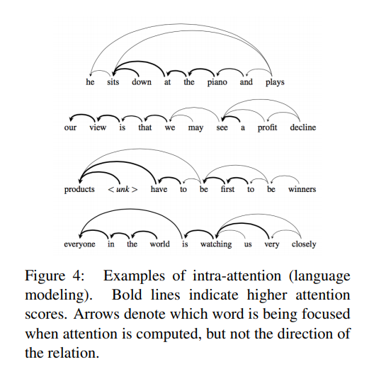
One of the key characteristics of the Transformer that differentiates from RNN Encoder-Decoder and its variants is the utilization of self-attention. Self-attention, or intra-attention, attempts to discover patterns among inputs in a single sequence, rather than input/output pairs from two sequences. This process, initially utilized by the Long Short-Term Memory Networks (Cheng et al. 2016), resembles the human reading process.

[Image source: Cheng et al. (2016)]

Since there is only one sequence to model, the query, key, and value are the same in self-attention networks ($Q = K = V$). Also, since there is no RNN cells in the network, they are not hidden states. Rather, they are positional-encoded embedded sequence inputs. We will see what positional encoding is in the following section, so don’t worry.

The self-attention mechanism is extremely powerful that the Transformer completely eschews traditional choices for sequence modeling, i.e., RNNs and CNNs. And this was such a revolutionary proposal that the authors dedicated an entire section (specifically, Section 4) advocating the use of self-attention. Below are three reasons that the authors opted for self-attention with feedforward layers.

One is the total computational complexity per layer. Another is the amount of computation that can be parallelized, as measured by the minimum number of sequential operations required. The third is the path length between long-range dependencies in the network (Vaswani et al. 2017, pp. 6)

Positional encoding

As the Transformer eschews CNN and RNN, additional information regarding the order of the sequence should be injected.

Since our model contains no recurrence and no convolution, in order for the model to make use of the order of the sequence, we must inject some information about the relative or absolute position of the tokens in the sequence. To this end, we add “positional encodings” to the input embeddings at the bottoms of the encoder and decoder stacks (Vaswani et al. 2017, pp. 5-6)

Among many choices for positional encoding, the authors used sine and cosine functions. For each position $pos$ in the sequence and dimension $i$, encodings are obtained with below functions.

[PE_{pos, 2i} = sin(\frac{pos}{10000^{2i/d_{model}}})]

[PE_{pos, 2i + 1} = cos(\frac{pos}{10000^{2i/d_{model}}})]

The dimension ($i$) spans through 1 to $d_{model}$, which is the dimensionality of the embedding space. Therefore, outputs from positional encoding have the same tensor size as the embedded sequences. They are added up and passed onto the next layer, which is multi-head attention.

Multi-head attention

Multi-head attention is basically concatenating multiple attention results and projecting it with linear transformation ($W^O$).

\begin{equation} MultiHead(Q, K, V) = Concat(head_1, head_2, …, head_h)W^O \end{equation}

To minimize the compuational cost, the query, key and value are projected to lower-dimensional space ($d_k, d_k, d_v$) with linear transformations ($W_i^Q, W_i^K, W_i^V$). It is claimed that the total computational cost is kept similar to that of single attention with full dimensionality.

\begin{equation} head_i = Attention(QW_i^Q, KW_i^K, VW_i^V) \end{equation}

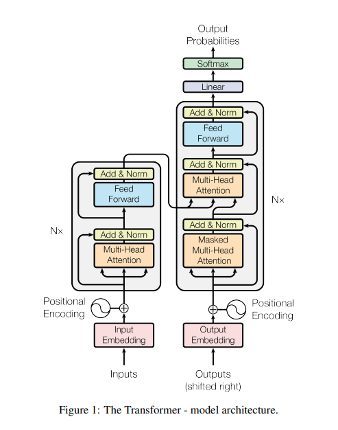
Finally, we have gone through all of the key building blocks of Transformer. Now you would be in a better position to understand the architecture of Transformer outlined in below figure by Vaswani et al. (2017). It is not required to entirely understand the mathematics and details of each mechanism (at least I can’t, to be honest), but good to have a general idea of how the network works.

[Image source: Vaswani et al. (2017)]
In the next posting, let’s try implementing the Transformer with Pytorch. Good new is that Pytorch provides nn.Transformer and related modules that makes implemenation extremely easy. See you in the next posting!

References