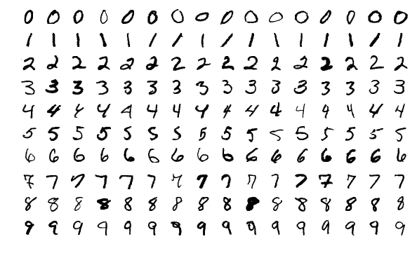
Buomsoo Kim

Using external fonts in Google Colaboratory (Google colab에서 한글 폰트 사용하기)

|

Using external fonts in Google colaboratory

In most cases, it is enough to use default font in Python programming, especially you are using English. But, mostly when visualizing results, languages other than English are to be used for the sake of communication, and you would like to use non-default fonts in Python.

When you are using local IDEs like PyCharm or Jupyter Notebook, this is not a difficult issue. You could just install font in your environment, and just let the visualization library (e.g., matplotlib) to know where the installed font in located.

However, when using Google Colab, this is kind of tricky as you do not use local runtime environment most of the time. Instead, you run Python program in the Ubuntu environment provided by the server. So, another way to install and use the external font should be employed to operate.

In this posting, I show you one of the easy way to solve this problem. I have made the example with one of the Korean fonts provided by Google (Noto Sans CJK KR), but if you just change the url and the name of font, you could virtually use any font you want!

0. Using other languages in colab without installation

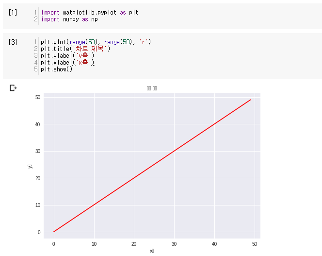
When I tried using Korean without installation, the result looked like this.
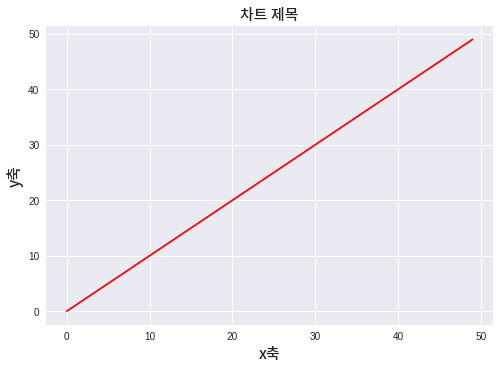
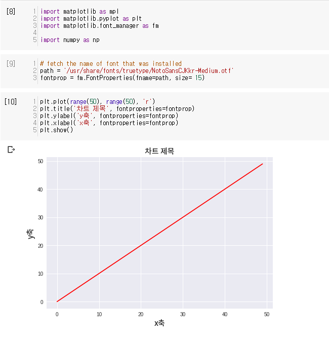
In the end, this chart will look like below (sorry for non-korean guys). Now let’s look at the procedure step by step.
1. Obtain the source (url) of the font

To start with, you wil have to obtain the source of the external font you are trying to use. In my case, I will use Noto Sans font provided by Google.

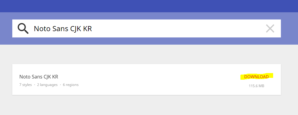
You could find Google Noto Fonts here

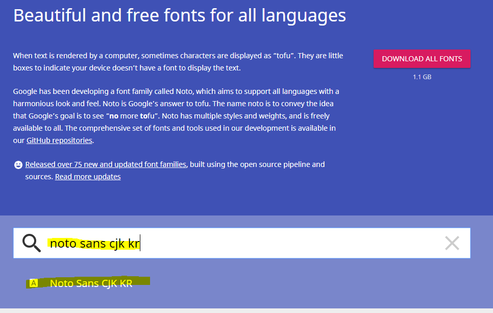
First, search for the font that you are going to use. As I mentioned, I have used Noto Sans CJK KR for my Korean letters.
Then, download and check if this is the font that you are going to use. And check the file names (mostly .otf or ttf for fonts) and remeber them. The name of the font file that I am going to use is NotoSansCJKkr-Medium.otf. Also, remember the download link of the zip file. In my case, it is https://noto-website-2.storage.googleapis.com/pkgs/NotoSansCJKkr-hinted.zip
3. Download font files

Now, open a google colab file and start coding. We are going to use google colab like a Ubuntu terminal for the moment. So, Ubuntu commands such as wget, mv, unzip are going to be used.

To start with, download the zip file (in this case, NotoSansCJKkr-hinted.zip) that contains font files.

!wget "source_of_your_target_file"

4. Unzip font files

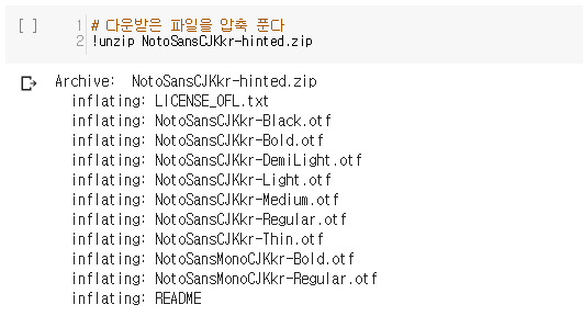
As you have checked, font files are contained in a zip file (.zip), so you have to unzip the file to get the font files. Use !unzip command to open the zip file.

Note that if you have downloaded font file itself (i.e., not zipped), you do not have to unzip them.

!unzip "your_file_name.zip"
5. Move font files

Now, move your font file to the font directory in Ubuntu environment. Use !mv command to move the file. In most cases you will get to move your font to /usr/share/fonts/truetype. Note that this will not do anything with your local environment!!!

!mv "your_font_file_name" "font_directory"

In my case,

!mv NotoSansCJKkr-Medium.otf /usr/share/fonts/truetype/

6. Test if it works properly

Now the installation is finished. I will test by using installed Korean font in drawing a chart with matplotlib libary.

import matplotlib as mpl
import matplotlib.pyplot as plt
import matplotlib.font_manager as fm

# fetch the name of font that was installed
path = '/usr/share/fonts/truetype/your_font_name'
fontprop = fm.FontProperties(fname=path)

In my case, I have used below code.

import matplotlib as mpl
import matplotlib.pyplot as plt
import matplotlib.font_manager as fm

path = '/usr/share/fonts/truetype/NotoSansCJKkr-Medium.otf'
fontprop = fm.FontProperties(fname=path, size= 15)

plt.plot(range(50), range(50), 'r')
plt.title('차트 제목', fontproperties=fontprop)
plt.ylabel('y축', fontproperties=fontprop)
plt.xlabel('x축', fontproperties=fontprop)
plt.show()
Code

Code in this post can be exhibited by below link. link

케라스와 함께하는 쉬운 딥러닝 (6) - 뉴럴 네트워크의 학습 과정 개선하기

|

다층 퍼셉트론 6 (Improving techniques for training neural networks 3)

Objective: 인공신경망 모델을 효율적으로 학습시키기 위한 개선 방법들에 대해 학습한다.

지지난 포스팅지난 포스팅에서 뉴럴 네트워크의 학습 과정을 개선하기 위한 아래의 여섯 가지 방법에 대해서 알아보았다.

  • 가중치 초기화(Weight Initialization)
  • 활성함수(Activation Function)
  • 최적화(Optimization)
  • 배치 정규화(Batch Normalization)
  • 드랍아웃(Dropout)
  • 앙상블(Model Ensemble)

여기에 덧붙여, 지난번 포스팅에서는 학습 시간을 단축시키기 위하여 1/3의 학습 데이터만 가지고 학습을 시켰는데, 이번 포스팅에서는 전체 학습데이터를 가지고 신경망 모델을 학습 후 검증해 보자.

MNIST 데이터 셋 불러오기

# 케라스에 내장된 mnist 데이터 셋을 함수로 불러와 바로 활용 가능하다
from keras.datasets import mnist
import matplotlib.pyplot as plt

(X_train, y_train), (X_test, y_test) = mnist.load_data()
plt.imshow(X_train[0])    # show first number in the dataset
plt.show()
print('Label: ', y_train[0])


plt.imshow(X_test[0])    # show first number in the dataset
plt.show()
print('Label: ', y_test[0])


데이터 셋 전처리

앞서 언급했다시피, MNIST 데이터는 흑백 이미지 형태로, 2차원 행렬(28 X 28)과 같은 형태라고 할 수 있다.


하지만 이와 같은 이미지 형태는 우리가 지금 활용하고자 하는 다층 퍼셉트론 모델에는 적합하지 않다. 다층 퍼셉트론은 죽 늘어놓은 1차원 벡터와 같은 형태의 데이터만 받아들일 수 있기 때문이다. 그러므로 우리는 28 X 28의 행렬 형태의 데이터를 재배열(reshape)해 784 차원의 벡터로 바꾼다.

from keras.utils.np_utils import to_categorical
from sklearn.model_selection import train_test_split

# reshaping X data: (n, 28, 28) => (n, 784)
X_train = X_train.reshape((X_train.shape[0], -1))
X_test = X_test.reshape((X_test.shape[0], -1))


# 타겟 변수를 one-hot encoding 한다
y_train = to_categorical(y_train)
y_test = to_categorical(y_test)

print(X_train.shape, X_test.shape, y_train.shape, y_test.shape)

아래에 보다시피 이번에는 6만개의 학습 데이터를 가지고 모델을 학습시키고, 1만개의 데이터를 가지고 학습 결과를 검증해 본다.

(60000, 784), (10000, 784), (60000,), (10000,)

모델 생성 및 학습

우리가 처음 생성해 보았던 Vanilla MLP와 어떻게 다른지 한번 비교해 보자.

def mlp_model():
    model = Sequential()

    model.add(Dense(50, input_shape = (784, ), kernel_initializer='he_normal'))   # 가중치 초기화 방식 변경
    model.add(BatchNormalization())     # 배치 정규화 레이어 추가
    model.add(Activation('relu'))       # 활성함수로 Relu 사용
    model.add(Dropout(0.2))             # 드랍아웃 레이어 추가
    model.add(Dense(50, kernel_initializer='he_normal'))
    model.add(BatchNormalization())
    model.add(Activation('relu'))    
    model.add(Dropout(0.2))
    model.add(Dense(50, kernel_initializer='he_normal'))
    model.add(BatchNormalization())
    model.add(Activation('relu'))
    model.add(Dropout(0.2))
    model.add(Dense(50, kernel_initializer='he_normal'))
    model.add(BatchNormalization())
    model.add(Activation('relu'))
    model.add(Dropout(0.2))
    model.add(Dense(10, kernel_initializer='he_normal'))
    model.add(Activation('softmax'))

    adam = optimizers.Adam(lr = 0.001)    # Adam optimizer 사용
    model.compile(optimizer = adam, loss = 'categorical_crossentropy', metrics = ['accuracy'])

    return model

앙상블 할 때 모델의 개수도 5개로 늘려본다.

# create 5 models to ensemble
model1 = KerasClassifier(build_fn = mlp_model, epochs = 100)
model2 = KerasClassifier(build_fn = mlp_model, epochs = 100)
model3 = KerasClassifier(build_fn = mlp_model, epochs = 100)
model4 = KerasClassifier(build_fn = mlp_model, epochs = 100)
model5 = KerasClassifier(build_fn = mlp_model, epochs = 100)

:
ensemble_clf = VotingClassifier(estimators = [('model1', model1), ('model2', model2), ('model3', model3), ('model4', model4), ('model5', model5)], voting = 'soft')
ensemble_clf.fit(X_train, y_train)

모델 평가

기본 모델에 배치정규화만 적용했음에도 불구하고 91.54%의 높은 정확도를 보인다. 앞으로 네트워크를 만들 때 배치 정규화는 웬만하면 적용해 주는 것이 좋다(논문에 따르면 뒤에서 나올 regularization의 효과도 있어 배치 정규화를 적용하면 드랍아웃을 적용하지 않아도 된다고 한다).

y_pred = ensemble_clf.predict(X_test)
print('Acc: ', accuracy_score(y_pred, y_test))
Acc:  0.9801

최종 결과로 98%가 넘는 높은 정확도를 기록하였다. 모델 구조(복잡도나 크기)는 바꾸지 않았음에도 불구하고 아무런 개선 사항도 적용하지 않은 Vanilla MLP가 20% 정도의 정확도를 기록했던 것과 비교하면 괄목할 만한 성과이다.

일반적으로 뉴럴 네트워크를 학습시킬 때에는 여기서 나온 7가지 학습 개선 방법(가중치 초기화, 활성함수, 최적화, 배치 정규화, 드랍아웃, 앙상블, 학습 데이터 추가)을 모두 총동원하여 정확도(혹은 정밀도, 재현율, ROC 등)를 조금이라도 높이기 위해서 노력한다. 즉, 최소한 현업에 적용할 만한 뉴럴 네트워크를 만들 때 여기서 나온 방법은 모두 활용을 해볼만한 가치가 있다는 얘기다. 물론 어떤 상황에 어떤 방식이 유효할지는 그때그때 다르기 때문에 최적화된 결과를 위해서는 삽질을 통해 실험을 많이 해봐야 한다… (데이터 사이언스의 8할은 노가다이다)

이제 다음 포스팅에서는 이미지 데이터를 학습하는 데 최적화된 모델로 알려져 있는 합성곱 신경망(CNN; Convolutional Neural Networks)에 대해서 알아 보자!

전체 코드

본 실습의 전체 코드는 여기에서 열람하실 수 있습니다!

케라스와 함께하는 쉬운 딥러닝 (5) - 뉴럴 네트워크의 학습 과정 개선하기

|

다층 퍼셉트론 5 (Improving techniques for training neural networks 2)

Objective: 인공신경망 모델을 효율적으로 학습시키기 위한 개선 방법들에 대해 학습한다.

  • 배치 정규화(Batch Normalization)
  • 드랍아웃(Dropout)
  • 앙상블(Model Ensemble)

지난 포스팅에서 뉴럴 네트워크의 학습 과정을 개선하기 위한 방법으로 가중치 초기화, 활성함수, 최적화에 대해서 알아보았다. 세개 다 최근 10년 간 인공지능 연구자들이 꾸준히 연구해온 분야이며, 괄목할 만한 발전이 있었던 분야이다. 이번 글에서 알아볼 세 가지 방법(배치 정규화, 드랍아웃, 모델 앙상블)도 매우 중요한 개념이며 현대 인공 신경망 모델의 필수적인 요소이다.

MNIST 데이터 셋 불러오기

# 케라스에 내장된 mnist 데이터 셋을 함수로 불러와 바로 활용 가능하다
from keras.datasets import mnist
import matplotlib.pyplot as plt

(X_train, y_train), (X_test, y_test) = mnist.load_data()
plt.imshow(X_train[0])    # show first number in the dataset
plt.show()
print('Label: ', y_train[0])


plt.imshow(X_test[0])    # show first number in the dataset
plt.show()
print('Label: ', y_test[0])


데이터 셋 전처리

앞서 언급했다시피, MNIST 데이터는 흑백 이미지 형태로, 2차원 행렬(28 X 28)과 같은 형태라고 할 수 있다.


하지만 이와 같은 이미지 형태는 우리가 지금 활용하고자 하는 다층 퍼셉트론 모델에는 적합하지 않다. 다층 퍼셉트론은 죽 늘어놓은 1차원 벡터와 같은 형태의 데이터만 받아들일 수 있기 때문이다. 그러므로 우리는 28 X 28의 행렬 형태의 데이터를 재배열(reshape)해 784 차원의 벡터로 바꾼다.

from keras.utils.np_utils import to_categorical
from sklearn.model_selection import train_test_split

# reshaping X data: (n, 28, 28) => (n, 784)
X_train = X_train.reshape((X_train.shape[0], -1))
X_test = X_test.reshape((X_test.shape[0], -1))

# 학습 과정을 단축시키기 위해 학습 데이터의 1/3만 활용한다
X_train, _ , y_train, _ = train_test_split(X_train, y_train, test_size = 0.67, random_state = 7)

# 타겟 변수를 one-hot encoding 한다
y_train = to_categorical(y_train)
y_test = to_categorical(y_test)

print(X_train.shape, X_test.shape, y_train.shape, y_test.shape)
(19800, 784) (10000, 784) (19800, 10) (10000, 10)

배치 정규화(Batch Normalization)

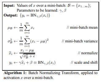
간단히 얘기해서 배치 정규화는 인공신경망에 입력값을 평균 0, 분산 1로 정규화(normalize)해 네트워크의 학습이 잘 일어나도록 돕는 방식이다. 앞에서 자세히 설명을 하지는 않았지만 배치(batch)는 가중치 학습을 위해 경사하강법(gradient descent)을 적용할 때 모델이 입력을 받는 데이터의 청크(즉, 일부 데이터 인스턴스)이다.


케라스에서 모델을 학습할 때 fit()함수를 적용할 때 설정하는 batch_size 파라미터는 바로 이 데이터의 청크의 크기(개수)를 의미한다. 예를 들어 batch_size를 32로 적용하면 모델이 데이터 인스턴스를 32개 본 후에 가중치를 업데이트하는 것이며, 배치 정규화를 적용하면 각 32개의 데이터 인스턴스가 feature별로 정규화된다.

케라스에서 배치 정규화는 하나의 레이어(BatchNormalization())처럼 작동하며, 보통 Dense 혹은 Convolution 레이어와 활성함수(Activation) 레이어 사이에 들어간다.

모델 생성 및 학습

from keras.layers import BatchNormalization
def mlp_model():
    model = Sequential()

    model.add(Dense(50, input_shape = (784, )))
    model.add(BatchNormalization())                    # Add Batchnorm layer before Activation
    model.add(Activation('sigmoid'))    
    model.add(Dense(50))
    model.add(BatchNormalization())                    # Add Batchnorm layer before Activation
    model.add(Activation('sigmoid'))    
    model.add(Dense(50))
    model.add(BatchNormalization())                    # Add Batchnorm layer before Activation
    model.add(Activation('sigmoid'))    
    model.add(Dense(50))
    model.add(BatchNormalization())                    # Add Batchnorm layer before Activation
    model.add(Activation('sigmoid'))    
    model.add(Dense(10))
    model.add(Activation('softmax'))

    sgd = optimizers.SGD(lr = 0.001)
    model.compile(optimizer = sgd, loss = 'categorical_crossentropy', metrics = ['accuracy'])

    return model
model = mlp_model()
history = model.fit(X_train, y_train, validation_split = 0.3, epochs = 100, verbose = 0)

모델 학습 결과 시각화


모델 평가

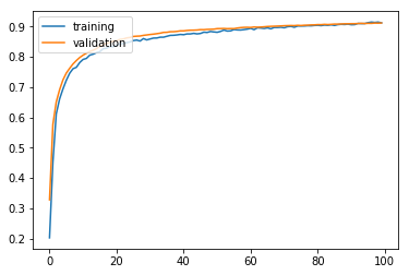
기본 모델에 배치정규화만 적용했음에도 불구하고 91.54%의 높은 정확도를 보인다. 앞으로 네트워크를 만들 때 배치 정규화는 웬만하면 적용해 주는 것이 좋다(논문에 따르면 뒤에서 나올 regularization의 효과도 있어 배치 정규화를 적용하면 드랍아웃을 적용하지 않아도 된다고 한다).

results = model.evaluate(X_test, y_test)
print('Test accuracy: ', results[1])
Test accuracy:  0.9154

드랍아웃(Dropout)

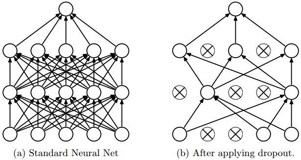
드랍아웃은 앞서 배치 정규화에서 잠깐 언급했던 regularization의 효과를 위한 방법이다. 아이디어 자체는 굉장히 단순하다. 어떤 레이어에 드랍아웃을 적용하면, 그 레이어의 모든 노드에서 나가는 activation을 특정 확률로 지워버린다.


이렇게 간단한 아이디어가 왜 필요하냐고 물어볼 수 있겠지만, 그 이유는 역설적이게도 뉴럴 네트워크가 너무 똑똑해지는(기억력이 좋아지는) 것을 방지하는 것이다. 예를 들어, 토익 시험을 본다고 생각을 하자. 연습 문제를 가지고 공부를 하는데 연습 문제의 리스닝 셋에서 강아지 사진이 있는 문제의 답이 모두 C라고 가정하자. 어떤 학생이 연습 문제를 가지고 너무 공부를 열심히 한 나머지 강아지 사진이 있는 문제의 답은 C라고 외워버리게 되고, 실전에서 강아지 문제가 나오자 마자 답을 C로 찍어버렸는데 사실 그 문제의 답은 D였던 것이다. 제 3자가 보면 말도 안되는 이야기지만 학생 입장에서는 공부를 정말 열심히해서 연습 문제의 답까지 외워버렸는데 막상 실전에 가서 문제를 틀려버린 상황이 된 것이다.

이것이 바로 학습 데이터에 대한 “과적합(overfitting)” 문제이며, 드랍아웃은 이러한 상황을 방지하기 위한 장치이다. 일부러 모델을 학습할 때 일부 노드의 activation을 지워버려 다소 “멍청한(기억력이 떨어지는)” 모델을 만들어 문제에 대한 과적합(overfitting)을 막는다. 물론 검증할 때에는 모든 activation을 다시 살린다(실전에 가서는 모든 기억력을 총동원하는 것처럼…).

우리 예에서는 드랍아웃이 의미가 없을 수 있겠으나, ResNet과 같이 복잡하고 거대한 모델을 만들 때 드랍아웃은 유의미한 성능을 발휘한다. 모델이 “딥(deep)”해지면 해질수록 데이터에 대한 학습 과적합이 일어나기 십상이기 때문에, 이러한 경우 드랍아웃을 통해 과적합을 줄이고 검증 정확도를 높일 수 있다.

모델을 만들었는데 학습 정확도가 검증 정확도에 비해 지나치게 높으면 늘 과적합을 의심하고 드랍아웃을(혹은 유사한 효과를 갖는다고 하는 배치 정규화를) 적용해 보자.

케라스에서 드랍아웃을 적용할 때에는 일반적으로 활성 함수(Activation) 레이어 뒤에 붙이며, 인자로 activation을 드랍할 확률인 dropout_rate를 설정해 주어야 한다.

모델 생성 및 학습

from keras.layers import Dropout
def mlp_model():
    model = Sequential()

    model.add(Dense(50, input_shape = (784, )))
    model.add(Activation('sigmoid'))    
    model.add(Dropout(0.2))                       
    model.add(Dense(50))
    model.add(Activation('sigmoid'))
    model.add(Dropout(0.2))                      
    model.add(Dense(50))
    model.add(Activation('sigmoid'))    
    model.add(Dropout(0.2))                        
    model.add(Dense(50))
    model.add(Activation('sigmoid'))    
    model.add(Dropout(0.2))                        
    model.add(Dense(10))
    model.add(Activation('softmax'))

    sgd = optimizers.SGD(lr = 0.001)
    model.compile(optimizer = sgd, loss = 'categorical_crossentropy', metrics = ['accuracy'])

    return model
model = mlp_model()
history = model.fit(X_train, y_train, validation_split = 0.3, epochs = 100, verbose = 0)

모델 학습 결과 시각화

앞서 말했다시피, 우리 모델은 복잡한 모델이 아니기 때문에 과적합이 일어나지 않았고, 드랍아웃이 이 상황에서는 의미가 없다. 오히려 정확도를 감소시킨다.


모델 평가

기본 모델에 비해 test accuracy가 낮아졌다. 원래 학습 데이터를 가지고 공부를 제대로 하지 않은 애한테 공부한 시간을 빼앗은 꼴이다..

results = model.evaluate(X_test, y_test)
print('Test accuracy: ', results[1])
Test accuracy:  0.1135

앙상블(Model Ensemble)

모델 앙상블 또한 매우 강력한 개념이다. CS231n 강좌에 따르면, 모델 앙상블을 적절하게 하면 웬만하면 정확도가 1~2% 정도는 올라간다고 한다. 원래 머신러닝에서 앙상블하는 것도 bootstrapping, bagging 등 여러 가지 방법이 있는 것처럼 뉴럴 네트워크의 앙상블도 여러 가지 방법이 있다. 자세한건 여기를 참조하자.

앙상블이 효과를 발휘하는 이유를 간단히 설명하자면, 네트워크를 학습할 때 마다 가중치 초기값이 조금씩 달라 결과가 조금씩 달라진다. 이에 따라 어느 정도의 randomness를 가지고 모델마다 결과가 미묘하게 달라진다(차이의 크기는 데이터, 네트워크 마다 다름). 앙상블은 이처럼 서로 다른 모델들을 합쳐 일종의 “집단지성(collective intelligence)”을 발휘하여 각기 하나의 모델보다 나은 최종 모델을 만들어 낸다. 요약하자면 “백지장도 맞들면 낫다” 정도.

앙상블을 할 때에는 일반적으로 멍청한 모델(underfitting)이 똑똑한 모델(overfitting)보다 낫고, 모델 간의 차이가 크면 클수록 좋다. 물론 일반론이므로 결과는 항상 돌려봐야만 확인할 수 있다. (CS231n에서 배운 것과는 다르게 앙상블 했는데 정확도 개선이 전혀 없는경우도 있다…)

모델 생성 및 학습

scikit-learn에 있는 VotingClassifier를 적용해보자. 서로 다른 모델을 합쳐서 결과값을 다수결로 결정한다(voting).

import numpy as np
from keras.wrappers.scikit_learn import KerasClassifier
from sklearn.ensemble import VotingClassifier
from sklearn.metrics import accuracy_score

def mlp_model():
    model = Sequential()

    model.add(Dense(50, input_shape = (784, )))
    model.add(Activation('sigmoid'))    
    model.add(Dense(50))
    model.add(Activation('sigmoid'))    
    model.add(Dense(50))
    model.add(Activation('sigmoid'))    
    model.add(Dense(50))
    model.add(Activation('sigmoid'))    
    model.add(Dense(10))
    model.add(Activation('softmax'))

    sgd = optimizers.SGD(lr = 0.001)
    model.compile(optimizer = sgd, loss = 'categorical_crossentropy', metrics = ['accuracy'])

    return model

# 서로 다른 모델을 3개 만들어 합친다
model1 = KerasClassifier(build_fn = mlp_model, epochs = 100, verbose = 0)
model2 = KerasClassifier(build_fn = mlp_model, epochs = 100, verbose = 0)
model3 = KerasClassifier(build_fn = mlp_model, epochs = 100, verbose = 0)
ensemble_clf = VotingClassifier(estimators = [('model1', model1), ('model2', model2), ('model3', model3)], voting = 'soft')
ensemble_clf.fit(X_train, y_train)
y_pred = ensemble_clf.predict(X_test)

모델 평가

다행히도(?) 우리 모델에서는 3개 합치자 정확도가 조금 올라갔다.

print('Test accuracy:', accuracy_score(y_pred, y_test))
Test accuracy: 0.3045

이번 포스팅에서는 뉴럴 네트워크의 학습 과정을 개선시킬 수 있는 나머지 세 가지 방식에 대해 알아봤다. 뉴럴 네트워크와 관련하여 연구가 계속 지속되고 있는 만큼, 이 외에도 모델을 개선할 수 있는 방법이 수많이 존재하고 모델마다 적합한 방식이 다르다. 이처럼 실험해야 될 경우의 수가 많아질수록 케라스와 같은 high-level API가 강점을 발휘하는 것이 아닐까 싶다. 코드를 모듈화하고 파라미터를 조금씩만 바꾸어가면서 여러 가지 테스팅을 최대한 많이 해보는 것이 현실에서 데이터 마이닝 문제를 풀 때 가장 좋은 접근법이라고 생각한다.

전체 코드

본 실습의 전체 코드는 여기에서 열람하실 수 있습니다!

케라스와 함께하는 쉬운 딥러닝 (4) - 뉴럴 네트워크의 학습 과정 개선하기

|

다층 퍼셉트론 4 (Improving techniques for training neural networks)

Objective: 인공신경망 모델을 효율적으로 학습시키기 위한 개선 방법들에 대해 학습한다.

  • 가중치 초기화(Weight Initialization)
  • 활성함수(Activation Function)
  • 최적화(Optimization)

MNIST 데이터 셋 불러오기

# 케라스에 내장된 mnist 데이터 셋을 함수로 불러와 바로 활용 가능하다
from keras.datasets import mnist
import matplotlib.pyplot as plt

(X_train, y_train), (X_test, y_test) = mnist.load_data()
plt.imshow(X_train[0])    # show first number in the dataset
plt.show()
print('Label: ', y_train[0])


plt.imshow(X_test[0])    # show first number in the dataset
plt.show()
print('Label: ', y_test[0])


데이터 셋 전처리

앞서 언급했다시피, MNIST 데이터는 흑백 이미지 형태로, 2차원 행렬(28 X 28)과 같은 형태라고 할 수 있다.


하지만 이와 같은 이미지 형태는 우리가 지금 활용하고자 하는 다층 퍼셉트론 모델에는 적합하지 않다. 다층 퍼셉트론은 죽 늘어놓은 1차원 벡터와 같은 형태의 데이터만 받아들일 수 있기 때문이다. 그러므로 우리는 28 X 28의 행렬 형태의 데이터를 재배열(reshape)해 784 차원의 벡터로 바꾼다.

from keras.utils.np_utils import to_categorical
from sklearn.model_selection import train_test_split

# reshaping X data: (n, 28, 28) => (n, 784)
X_train = X_train.reshape((X_train.shape[0], -1))
X_test = X_test.reshape((X_test.shape[0], -1))

# 학습 과정을 단축시키기 위해 학습 데이터의 1/3만 활용한다
X_train, _ , y_train, _ = train_test_split(X_train, y_train, test_size = 0.67, random_state = 7)

# 타겟 변수를 one-hot encoding 한다
y_train = to_categorical(y_train)
y_test = to_categorical(y_test)

print(X_train.shape, X_test.shape, y_train.shape, y_test.shape)
(19800, 784) (10000, 784) (19800, 10) (10000, 10)

기본 MLP 모델 학습 및 평가

지난 세션에서 보았듯이, 아무런 개선을 거치지 않은 기본 MLP 모델에 MNIST 데이터를 학습하였을 때에는 21%라는 그리 훌륭하지 않은 결과가 나왔다.

모델 학습 결과 시각화

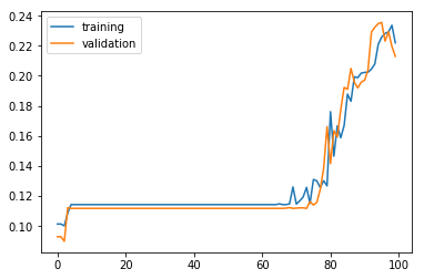
학습이 진행됨에 따라 달라지는 학습 정확도와 검증 정확도의 추이를 시각화해 본다. 60 에포크가 지난 후에 정확도가 올라가기 시작한다.

plt.plot(history.history['acc'])
plt.plot(history.history['val_acc'])
plt.legend(['training', 'validation'], loc = 'upper left')
plt.show()


모델 평가

results = model.evaluate(X_test, y_test)
print('Test accuracy: ', results[1])

학습 정확도 21.44%로 랜덤하게 찍는 경우의 예상 정확도(10%)보다는 높게 나왔지만, 그리 만족스러운 수치는 아니다.

Test accuracy:  0.2144

이제 어떻게 우리의 인공 신경망 모델의 MNIST 데이터에 대한 학습을 개선시킬 수 있는지 알아보자!

가중치 초기화(weight initialization)

가중치 초기화 방법을 따로 설정해 주지 않으면 기본적으로 케라스 레이어의 가중치 초기화 방식은 일정 구간 내에서 랜덤하게 찍는 random_uniform이다. 하지만 이러한 방식은 오차 역전파(back propagation) 과정에서 미분한 gradient가 지나치게 커지거나(exploding gradient) 소실되는(vanishing gradient) 문제에 빠질 위험성이 크다(자세한 내용은 여기 참고).

따라서, 어떻게 가중치를 초기화할 것인가에 대한 지속적인 연구가 진행되어 왔고, 이전에 비해 개선된 초기화 방식이 제안되었으며 널리 활용되고 있다. 케라스에서 제공하는 초기화 방식 중 흔히 사용되는 것들은 다음과 같다.

  • LeCun 초기화(lecun_uniform, lecun_normal): 98년도에 얀 르쿤이 제기한 방법으로 최근에는 Xavier나 He 초기화 방식에 비해 덜 사용되는 편이다.
  • Xavier 초기화(glorot_uniform, glorot_normal): 케라스에서는 glorot이라는 이름으로 되어있는데, 일반적으로는 Xavier Initialization이라고 알려져 있다. 사실 초기화 방식이 제안된 논문의 1저자 이름이 Xavier Glorot이다(출처). 2저자는 유명한 Yoshua Bengio.
  • He 초기화(he_uniform, he_normal): ResNet으로도 유명한 마이크로소프트(현재는 Facebook)의 Kaiming He가 2015년에 제안한 가장 최신의 초기화 방식이다. 수식을 보면 Xavier Initialization을 조금 개선한 것인데, 경험적으로 더 좋은 결과를 내었다고 한다.

모델 생성 및 학습

# 이제부터는 함수를 만들어 모델을 생성한다. 이렇게 하면 모듈화와 캡슐화가 되어 관리하기가 훨씬 쉽다.
def mlp_model():
    model = Sequential()
    
    model.add(Dense(50, input_shape = (784, ), kernel_initializer='he_normal'))     # use he_normal initializer
    model.add(Activation('sigmoid'))    
    model.add(Dense(50, kernel_initializer='he_normal'))                            # use he_normal initializer
    model.add(Activation('sigmoid'))    
    model.add(Dense(50, kernel_initializer='he_normal'))                            # use he_normal initializer
    model.add(Activation('sigmoid'))    
    model.add(Dense(50, kernel_initializer='he_normal'))                            # use he_normal initializer
    model.add(Activation('sigmoid'))    
    model.add(Dense(10, kernel_initializer='he_normal'))                            # use he_normal initializer
    model.add(Activation('softmax'))
    
    sgd = optimizers.SGD(lr = 0.001)
    model.compile(optimizer = sgd, loss = 'categorical_crossentropy', metrics = ['accuracy'])
    
    return model
model = mlp_model()
history = model.fit(X_train, y_train, validation_split = 0.3, epochs = 100, verbose = 0)

모델 학습 결과 시각화

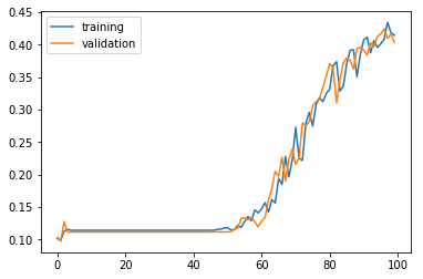
기존 모델과 비슷하게 60 에포크 이후로 정확도가 올라가기 시작하지만, 한번 탄력을 받자 훨씬 빠르게 올라간다.


모델 평가

역시 최종 test accuracy도 41%로 기본 모델에 비해 2배 정도 되는 수치를 보인다.

results = model.evaluate(X_test, y_test)
print('Test accuracy: ', results[1])
Test accuracy:  0.4105

활성함수(Activation Function)

기본 모델에서는 활성함수로 시그모이드 함수(sigmoid function)를 활용하였다. 하지만 시그모이드 함수의 경우 입력값이 조금만 커지거나 작아져도 곡선이 평평해져 기울기가 0에 가까워 지는것을 볼 수 있다. 이렇게 되면 랜덤 초기화 방식과 비슷하게 gradient가 소실되는 문제가 발생한다(용어때문에 헷갈리면 기울기 = 미분값 = gradient라고 생각하면 편하다).


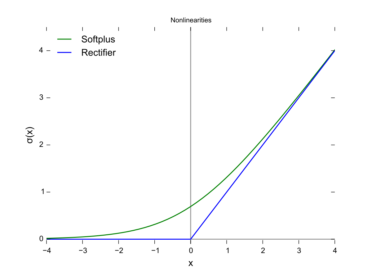
조금 다르지만 비슷하게 생긴 탄젠트 하이퍼볼릭(tanh) 함수도 비슷한 문제를 겪으며, 이를 해결하기 위해 나온 함수가 2013년 AlexNet과 함께 혜성처럼 등장한 ReLU (Rectified Linear Unit) 함수이다. 입력값이 0보다 크면 그대로, 0보다 작으면 0으로 출력을 내보내는 어찌보면 무식한(?) 형태이지만 gradient 소실 문제가 발생할 확률을 대폭 줄여주기 때문에 현재 가장 널리 활용되고 있는 활성함수이다. ReLU를 조금 변형한 PReLU, Leaky ReLU, SeLU 등도 제안되었지만, ReLU만큼 자주 사용되지는 않는다.


모델 생성 및 학습

def mlp_model():
    model = Sequential()
    
    model.add(Dense(50, input_shape = (784, )))
    model.add(Activation('relu'))    # use relu
    model.add(Dense(50))
    model.add(Activation('relu'))    # use relu
    model.add(Dense(50))
    model.add(Activation('relu'))    # use relu
    model.add(Dense(50))
    model.add(Activation('relu'))    # use relu
    model.add(Dense(10))
    model.add(Activation('softmax'))
    
    sgd = optimizers.SGD(lr = 0.001)
    model.compile(optimizer = sgd, loss = 'categorical_crossentropy', metrics = ['accuracy'])
    
    return model
model = mlp_model()
history = model.fit(X_train, y_train, validation_split = 0.3, epochs = 100, verbose = 0)

모델 학습 결과 시각화

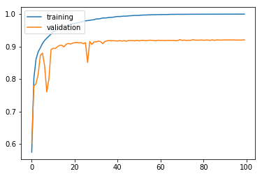
학습이 이전에 비해 굉장히 빨리되는 것을 볼 수 있다. 학습이 10바퀴 돌기도 전에 학습 오차가 10% 이내로 줄어들며 60 에포크쯤 가서는 학습 오차는 0에 가까워진다.


모델 평가

역시 최종 test accuracy도 92%로 이전 모델에 비해 비약적으로 높아진 것을 알 수 있다.

results = model.evaluate(X_test, y_test)
print('Test accuracy: ', results[1])
Test accuracy:  0.9208

최적화(Optimization)

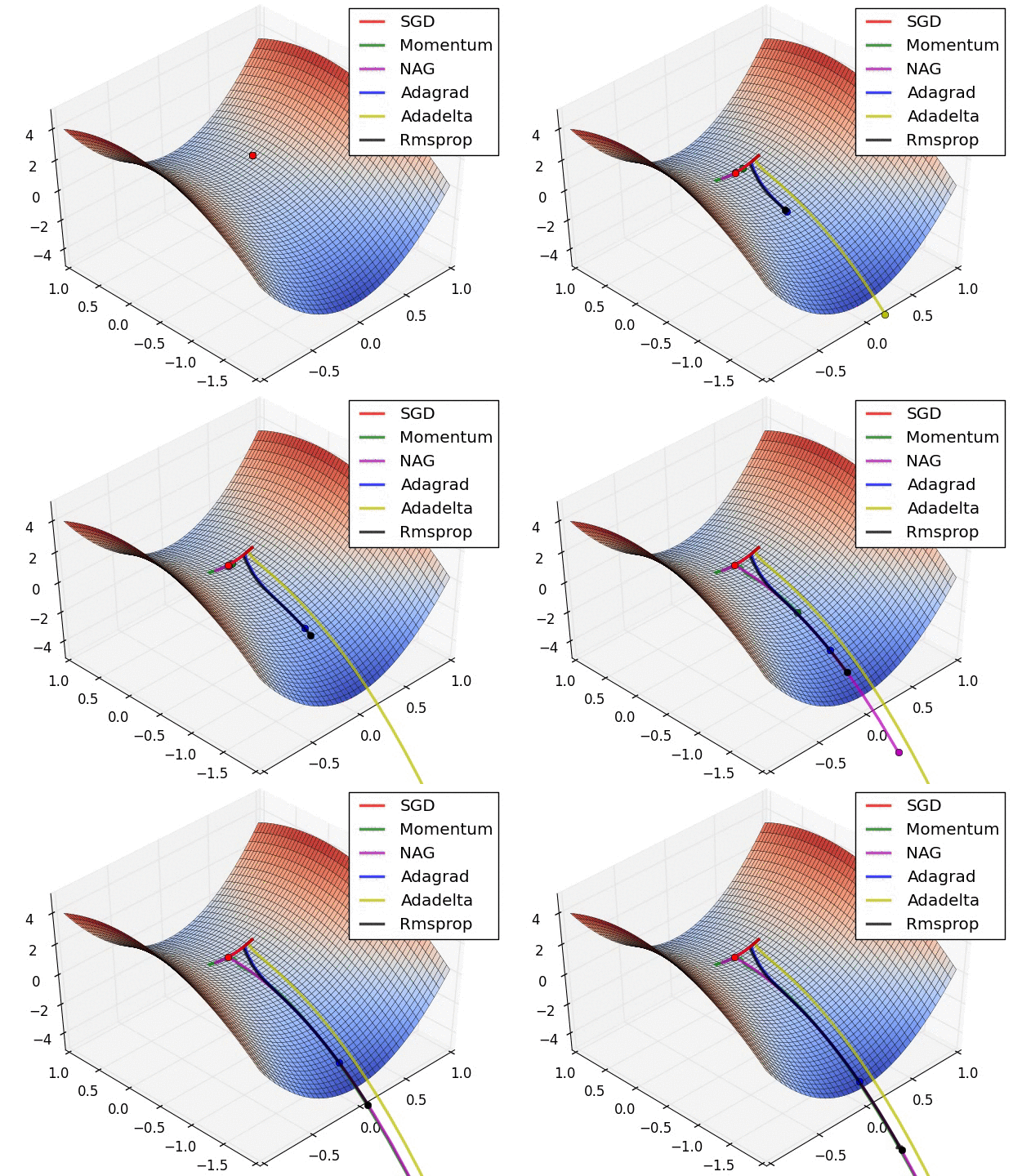
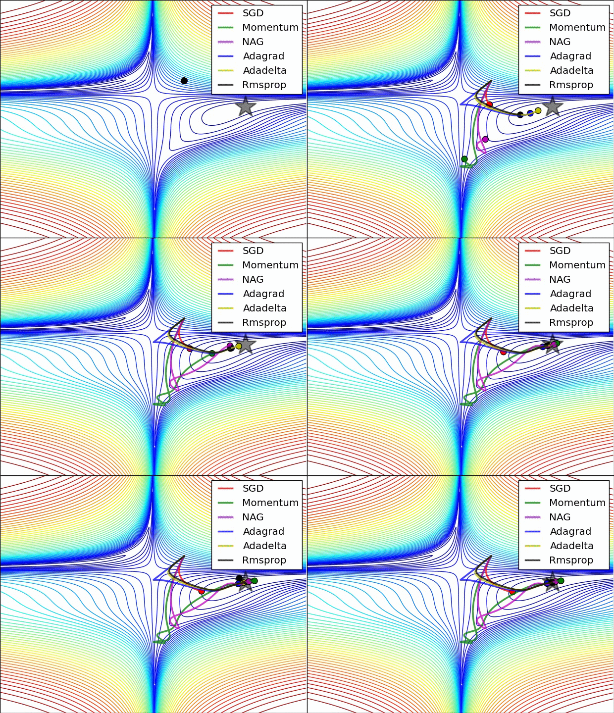
오차 역전파를 활용하는 뉴럴 네트워크의 최적화 방식으로 대부분 경사하강법(SGD; Stochastic Gradient Descent)를 활용한다. 그렇지만 SGD에도 수많은 변용이 존재하며, 각각 장점과 단점을 가지고 있다. 경사하강법을 구현할 때 처음에 스텝의 크기인 learning rate를 설정해 주는데, learning rate를 상황에 따라 계속 변경하면서 학습을 진행하는 adaptive learning methods가 흔히 활용된다(그때그때 실정에 맞추어 스텝의 크기를 바꾸어주다보니 학습이 훨씬 빠르다).


최근에는 RMSprop이나 Adam (RMSprop에 모멘텀의 개념을 접합한 optimizer)을 흔히 사용하며 케라스에서는 둘 다 지원된다.


모델 생성 및 학습

Adam을 써서 최적화를 해보자.

def mlp_model():
    model = Sequential()
    
    model.add(Dense(50, input_shape = (784, )))
    model.add(Activation('sigmoid'))    
    model.add(Dense(50))
    model.add(Activation('sigmoid'))  
    model.add(Dense(50))
    model.add(Activation('sigmoid'))    
    model.add(Dense(50))
    model.add(Activation('sigmoid'))    
    model.add(Dense(10))
    model.add(Activation('softmax'))
    
    adam = optimizers.Adam(lr = 0.001)                     # use Adam optimizer
    model.compile(optimizer = adam, loss = 'categorical_crossentropy', metrics = ['accuracy'])
    
    return model
model = mlp_model()
history = model.fit(X_train, y_train, validation_split = 0.3, epochs = 100, verbose = 0)

모델 학습 결과 시각화

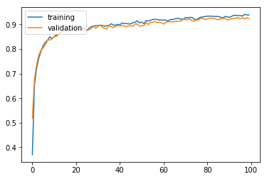
이번에도 학습이 이전에 비해 굉장히 빨리될 뿐 아니라, 학습/검증 정확도의 증가가 안정적으로 이루어지는 것을 볼 수 있다. 50에포크쯤 가서 90% 이상의 정확도에 안착하는 것을 볼 수 있다.


모델 평가

역시 최종 test accuracy도 92%로 이전 모델에 비해 비약적으로 높아진 것을 알 수 있다.

results = model.evaluate(X_test, y_test)
print('Test accuracy: ', results[1])
Test accuracy:  0.9248

이번 포스팅에서는 뉴럴 네트워크의 학습 과정을 개선시킬 수 있는 세 가지 방식에 대해 알아봤으며, 이를 적용해본 결과 92%라는 이전에 비해 훨씬 높은 검증 정확도를 얻을 수 있었다. 이처럼 케라스에서 코드를 몇 줄 바꾸는 간단한 과정으로 비약적인 정도의 개선과 변화를 가지고 올 수 있다는 것이 케라스의 가장 큰 장점이 아닌가 싶다.

다음 포스팅에서는 학습 과정을 개선시키는 3가지 방식에 대해서 더 알아보자.

전체 코드

본 실습의 전체 코드는 여기에서 열람하실 수 있습니다!

케라스와 함께하는 쉬운 딥러닝 (3) - 다층 퍼셉트론 3 (Training MLP with MNIST Dataset)

|

다층 퍼셉트론 3 (Training MLP with MNIST Dataset)

Objective: MNIST 데이터 셋을 불러와 이를 다층 퍼셉트론 모델에 적합한 형태로 변형하여 학습시킨다.

MNIST 데이터 셋

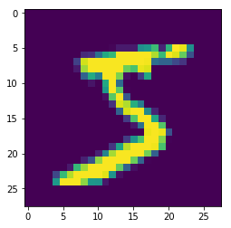
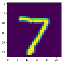
인공신경망에 대해 배울 때 흔히 사용되는 토이 데이터 셋(toy dataset) 중 하나며, 사람들이 직접 손으로 쓴 0부터 9까지의 숫자를 이미지화한 데이터이다. 6만 개의 학습 데이터와 1만 개의 검증 데이터로 구축되어 있다.


MNIST 데이터 셋 불러오기

# 케라스에 내장된 mnist 데이터 셋을 함수로 불러와 바로 활용 가능하다
from keras.datasets import mnist
import matplotlib.pyplot as plt

(X_train, y_train), (X_test, y_test) = mnist.load_data()
plt.imshow(X_train[0])    # show first number in the dataset
plt.show()
print('Label: ', y_train[0])


plt.imshow(X_test[0])    # show first number in the dataset
plt.show()
print('Label: ', y_test[0])


데이터 셋 전처리

앞서 언급했다시피, MNIST 데이터는 흑백 이미지 형태로, 2차원 행렬(28 X 28)과 같은 형태라고 할 수 있다.


하지만 이와 같은 이미지 형태는 우리가 지금 활용하고자 하는 다층 퍼셉트론 모델에는 적합하지 않다. 다층 퍼셉트론은 죽 늘어놓은 1차원 벡터와 같은 형태의 데이터만 받아들일 수 있기 때문이다. 그러므로 우리는 28 X 28의 행렬 형태의 데이터를 재배열(reshape)해 784 차원의 벡터로 바꾼다.

from keras.utils.np_utils import to_categorical
from sklearn.model_selection import train_test_split

# reshaping X data: (n, 28, 28) => (n, 784)
X_train = X_train.reshape((X_train.shape[0], -1))
X_test = X_test.reshape((X_test.shape[0], -1))

# 학습 과정을 단축시키기 위해 학습 데이터의 1/3만 활용한다
X_train, _ , y_train, _ = train_test_split(X_train, y_train, test_size = 0.67, random_state = 7)

# 타겟 변수를 one-hot encoding 한다
y_train = to_categorical(y_train)
y_test = to_categorical(y_test)

print(X_train.shape, X_test.shape, y_train.shape, y_test.shape)
(19800, 784) (10000, 784) (19800, 10) (10000, 10)

기본 MLP 모델 학습 및 평가

아무런 개선을 하지 않은 기본 MLP 모델(vanilla MLP)을 생성하여 학습해 본다.

모델 생성 및 학습

각 층의 뉴런의 개수는 50개인 은닉층(hidden layer) 4개를 가지고 있는 다층 퍼셉트론 구조를 생성한다.

from keras.models import Sequential
from keras.layers import Activation, Dense
from keras import optimizers

model = Sequential()
model.add(Dense(50, input_shape = (784, )))
model.add(Activation('sigmoid'))
model.add(Dense(50))
model.add(Activation('sigmoid'))
model.add(Dense(50))
model.add(Activation('sigmoid'))
model.add(Dense(50))
model.add(Activation('sigmoid'))
model.add(Dense(10))
model.add(Activation('softmax'))

sgd = optimizers.SGD(lr = 0.001)
model.compile(optimizer = sgd, loss = 'categorical_crossentropy', metrics = ['accuracy'])
history = model.fit(X_train, y_train, batch_size = 256, validation_split = 0.3, epochs = 100, verbose = 0)

모델 학습 결과 시각화

학습이 진행됨에 따라 달라지는 학습 정확도와 검증 정확도의 추이를 시각화해 본다. 60 에포크가 지난 후에 정확도가 올라가기 시작한다.

plt.plot(history.history['acc'])
plt.plot(history.history['val_acc'])
plt.legend(['training', 'validation'], loc = 'upper left')
plt.show()


모델 평가

results = model.evaluate(X_test, y_test)
print('Test accuracy: ', results[1])

학습 정확도 21.44%로 랜덤하게 찍는 경우의 예상 정확도(10%)보다는 높게 나왔지만, 그리 만족스러운 수치는 아니다.

Test accuracy:  0.2144

이미지 인식에 널리 활용되는 CNN (Convolutional Neural Networks) 구조를 활용한 현대 인공 신경망 모델은 MNIST 데이터 셋에서 정확도 99%가 넘는 완벽에 가까운 성능을 보여주고 있다. 그렇지만 아직 우리가 구현한 모델이 보이는 성능은 20%를 간신히 넘기는 수준이다.

이제 다음 포스팅에서 어떻게 우리의 인공 신경망 모델의 MNIST 데이터에 대한 학습을 개선시킬 수 있는지 알아보자.

전체 코드

본 실습의 전체 코드는 여기에서 열람하실 수 있습니다!