Buomsoo Kim

Attention in Neural Networks - 8. Alignment Models (1)

|

Attention Mechanism in Neural Networks - 8. Alignment Models (1)

So far, we looked into Seq2Seq, or the RNN Encoder-Decoder, proposed by Cho et al. (2014) and Sutskever et al. (2014). Seq2Seq is a powerful deep learning architecture to model variable-length sequence data. However, Bahdahanu et al. (2015) suggested one shortcoming of the need to compress all information from a souce sentence.

“A potential issue with this encoder–decoder approach is that a neural network needs to be able to compress all the necessary information of a source sentence into a fixed-length vector. This may make it difficult for the neural network to cope with long sentences, especially those that are longer than the sentences in the training corpus” (Bahdahanu et al. 2015)

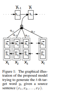
[Image source: Bahdahanu et al. (2015)]

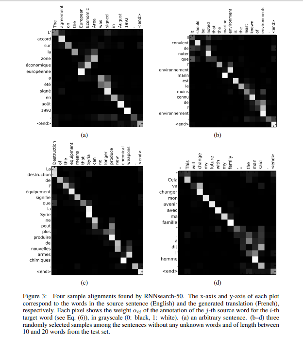
Such shortcoming leads to a potential loss of information, especially in case of long sentences as noted. Therefore, Bahdahanu et al. (2015) proposed an improve sequence-to-sequence architecture that aligns source and target sequences. This will enable the model to attend to a specific part of the source sentence, minimizing information loss from long sentences. In addition, such mechanism enables explanations of mapping between the source and target as in saliency maps below.

[Image source: Bahdahanu et al. (2015)]

In this posting, let’s briefly go through the alignment mechanism for input and output sequences proposed by Bahdahanu et al. (2015).

Encoder

The encoder is trained almost identically to the encoder in the Seq2Seq model. One slight difference is that the hidden state in each step in the source sequence should be memorized to align with the target sequence. $ h_t $ and $x_t$ are notations for the hidden state and source input at the step $t$. And the RNN in the encoder is noted as the function $f$. Therefore, each hidden state is calculated as below. Note that Bahdahanu et al. (2015) utilize bidirectional RNN to effectively model natural language sentences.

\begin{equation} h_t = f(x_t, h_{t-1}), t = 2, 3, …, n \end{equation}

Decoder

The decoder is slightly tweaked to align source and target states. To distiguish from the encoder, the hidden state and target output at the step $t$ are noted as $s_t$ and $y_t$. The context vector at each step is a weighted sum of the hidden states from the encoder.

\begin{equation} c_i = \sum_{j=1}^{n} \alpha_{ij}h_j \end{equation}

The weights at each step of the decoder is trained by a single dense layer applied by a softmax function to normalize the outputs.

\begin{equation} \begin{split} \alpha_{ij} = \frac{exp(e_{ij})}{\sum_{t=1}^{n}exp(e_{it})}
e_{ij} = dense(s_{i-1}, h_j) \end{split} \end{equation}

The dense layer here is an alignment model that aligns the source and target.

“an alignment model which scores how well the inputs around position j and the output at position i match.” (Bahdahanu et al. 2015)

In this posting, we briefly looked into the architecture of Seq2Seq with alignment proposed by Bahdahanu et al. (2015). From the next posting, let’s try implementing it with Pytorch. Thank you for reading.

References

Attention in Neural Networks - 7. Sequence-to-Sequence (Seq2Seq) (6)

|

Attention Mechanism in Neural Networks - 7. Sequence-to-Sequence (Seq2Seq) (6)

In the previous posting, we tried implementing another variant of the Seq2Seq model presented by Sutskever et al. (2014). Two key improvements in the variant, i.e., deep LSTM layers and reversing the order of input sequences, are claimed to significantly enhance the performances, especially in the existence of big data.

However, large data implies large computing and it often takes a huge amount of resources to train deep learning models, especially those having complicated structures such as Seq2Seq. There are many methods to expedite the learning process of large-scale deep learning models. One of the basic approaches is applying the mini-batch Stochastic Gradient Descent (SGD) to achieve faster iterations.

So far, we have trained and updated model weights after looking at one instance at a time. On another extreme, we can try updating the weights after looking the whole dataset. Naturally, this can be much faster in iterating, though with a lower convergence rate. In practice, we commonly choose to strike a balance between the two. In other words, we partition the training dataset in small chunks, i.e., “batches,” and update the weights after examining each batch.

Therefore, in this posting, we look into implemeting a mini-batch SGD version of the Seq2Seq model. This would be basically the same model as those in previous postings, but guarantees faster training. I acknowledge that I had a great help in converting the code from PyTorch Seq2Seq tutorials.

Import packages & download dataset

For mini-batch implementation, we take advantage of torch.utils.data to generate custom datasets and dataloaders. For more information, please refer to Generating Data in PyTorch

import re
import torch
import numpy as np
import torch.nn as nn

from matplotlib import pyplot as plt
from torch.utils.data.sampler import SubsetRandomSampler
from tqdm import tqdm

!wget https://www.manythings.org/anki/deu-eng.zip
!unzip deu-eng.zip

with open("deu.txt") as f:
  sentences = f.readlines()

# number of sentences
len(sentences)
204574

Data processing

One trick to easier mini-batch implementation of Seq2Seq, or any sequence models, is to set the length of sequences identical. By doing so, we can make mini-batch computation much easier, which is often three- or four-dimensional tensor multiplications. Here, I have set the maximum length of source and target sentences (MAX_SENT_LEN) to 10. Then, sentences that are shorter than 10 are padded with <pad> tokens and those longer than 10 are trimmed to fit in. However, note that doing so can lead to a loss of information due to trimming. If you want to evade such loss, you can set MAX_SENT_LEN to actual maximum length of source and target sentences. On the othe hand, this can be set arbitrarily. If you want faster computation despite the loss of information, you can set the value shorter than I did.

NUM_INSTANCES = 50000
MAX_SENT_LEN = 10
eng_sentences, deu_sentences = [], []
eng_words, deu_words = set(), set()
for i in tqdm(range(NUM_INSTANCES)):
  rand_idx = np.random.randint(len(sentences))
  # find only letters in sentences
  eng_sent, deu_sent = ["<sos>"], ["<sos>"]
  eng_sent += re.findall(r"\w+", sentences[rand_idx].split("\t")[0]) 
  deu_sent += re.findall(r"\w+", sentences[rand_idx].split("\t")[1])

  # change to lowercase
  eng_sent = [x.lower() for x in eng_sent]
  deu_sent = [x.lower() for x in deu_sent]
  eng_sent.append("<eos>")
  deu_sent.append("<eos>")

  if len(eng_sent) >= MAX_SENT_LEN:
    eng_sent = eng_sent[:MAX_SENT_LEN]
  else:
    for _ in range(MAX_SENT_LEN - len(eng_sent)):
      eng_sent.append("<pad>")

  if len(deu_sent) >= MAX_SENT_LEN:
    deu_sent = deu_sent[:MAX_SENT_LEN]
  else:
    for _ in range(MAX_SENT_LEN - len(deu_sent)):
      deu_sent.append("<pad>")

  # add parsed sentences
  eng_sentences.append(eng_sent)
  deu_sentences.append(deu_sent)

  # update unique words
  eng_words.update(eng_sent)
  deu_words.update(deu_sent)

The rest is identical. It is up to your choice to reverse the order of the source inputs or not. For more information refer to the previous posting.

eng_words, deu_words = list(eng_words), list(deu_words)

# encode each token into index
for i in tqdm(range(len(eng_sentences))):
  eng_sentences[i] = [eng_words.index(x) for x in eng_sentences[i]]
  deu_sentences[i] = [deu_words.index(x) for x in deu_sentences[i]]

idx = 10
print(eng_sentences[idx])
print([eng_words[x] for x in eng_sentences[idx]])
print(deu_sentences[idx])
print([deu_words[x] for x in deu_sentences[idx]])

You can see that short sentences are padded with <pad> as below.

[5260, 7633, 4875, 2214, 6811, 2581, 2581, 2581, 2581, 2581]
['<sos>', 'you', 'amuse', 'me', '<eos>', '<pad>', '<pad>', '<pad>', '<pad>', '<pad>']
[9284, 13515, 2514, 9574, 11982, 4432, 4432, 4432, 4432, 4432]
['<sos>', 'ihr', 'amüsiert', 'mich', '<eos>', '<pad>', '<pad>', '<pad>', '<pad>', '<pad>']

Setting parameters

One more parameter that is added is BATCH_SIZE. It is often set to values that are multiples of 16, e.g., 32, 64, 128, 256, 512, etc. However, this is also up to you. Just do not let it exceed total number of instances and consider the memory constraints of your GPU (or CPU)!

ENG_VOCAB_SIZE = len(eng_words)
DEU_VOCAB_SIZE = len(deu_words)
NUM_EPOCHS = 10
HIDDEN_SIZE = 128
EMBEDDING_DIM = 30
BATCH_SIZE = 128
LEARNING_RATE = 1e-2
DEVICE = torch.device('cuda') 

Dataset and Dataloader

We need to define the dataset and dataloader for efficient implementation of mini-batch SGD. In this posting, we randomly partition the dataset in 7-3 ratio and generate train and test dataloaders. For more information on this part, please refer to Generating Data in PyTorch

class MTDataset(torch.utils.data.Dataset):
  def __init__(self):
    # import and initialize dataset    
    self.source = np.array(eng_sentences, dtype = int)
    self.target = np.array(deu_sentences, dtype = int)
    
  def __getitem__(self, idx):
    # get item by index
    return self.source[idx], self.target[idx]
  
  def __len__(self):
    # returns length of data
    return len(self.source)

np.random.seed(777)   # for reproducibility
dataset = MTDataset()
NUM_INSTANCES = len(dataset)
TEST_RATIO = 0.3
TEST_SIZE = int(NUM_INSTANCES * 0.3)

indices = list(range(NUM_INSTANCES))

test_idx = np.random.choice(indices, size = TEST_SIZE, replace = False)
train_idx = list(set(indices) - set(test_idx))
train_sampler, test_sampler = SubsetRandomSampler(train_idx), SubsetRandomSampler(test_idx)

train_loader = torch.utils.data.DataLoader(dataset, batch_size = BATCH_SIZE, sampler = train_sampler)
test_loader = torch.utils.data.DataLoader(dataset, batch_size = BATCH_SIZE, sampler = test_sampler)

Encoder

The encoder is similary defined as previous postings. As we will be only needing the hidden state of the last GRU cell in the encoder, we reserve only the last h0 here. Also, note that the hidden state has size of (1, BATCH_SIZE, HIDDEN_SIZE) to incorporate batch learning.

class Encoder(nn.Module):
  def __init__(self, vocab_size, hidden_size, embedding_dim, device):
    super(Encoder, self).__init__()
    self.hidden_size = hidden_size
    self.vocab_size = vocab_size
    self.device = device
    self.embedding_dim = embedding_dim

    self.embedding = nn.Embedding(vocab_size, embedding_dim)
    self.gru = nn.GRU(embedding_dim, hidden_size)

  def forward(self, x, h0):
    # x = (BATCH_SIZE, MAX_SENT_LEN) = (128, 10)
    x = self.embedding(x)
    x = x.permute(1, 0, 2)
    # x = (MAX_SENT_LEN, BATCH_SIZE, EMBEDDING_DIM) = (10, 128, 30)
    out, h0 = self.gru(x, h0)
    print(out.shape)
    # out = (MAX_SENT_LEN, BATCH_SIZE, HIDDEN_SIZE) = (128, 10, 16)
    # h0 = (1, BATCH_SIZE, HIDDEN_SIZE) = (1, 128, 16)
    return out, h0

Decoder

The decoder is similarly trained but with a subtle difference of learning each step at a time. By doing so, we can save the output (x) and hidden state (h0) at every step.

class Decoder(nn.Module):
  def __init__(self, vocab_size, hidden_size, embedding_dim):
    super(Decoder, self).__init__()
    self.hidden_size = hidden_size
    self.vocab_size = vocab_size

    self.embedding = nn.Embedding(vocab_size, embedding_dim)
    self.gru = nn.GRU(embedding_dim, hidden_size)
    self.dense = nn.Linear(hidden_size, vocab_size)
    self.softmax = nn.LogSoftmax(dim = 1)
  
  def forward(self, x, h0):
    # x = (BATCH_SIZE) = (128)
    x = self.embedding(x).unsqueeze(0)
    # x = (1, BATCH_SIZE, EMBEDDING_DIM) = (1, 128, 30)
    x, h0 = self.gru(x, h0)
    x = self.dense(x.squeeze(0))
    x = self.softmax(x)
    return x, h0

Seq2Seq model

Here, we define the Seq2Seq model in a separate Python class. The first input to the Seq2Seq model is the token at the first timestep, i.e., “". We can designate this by slicing the ```target``` variable.

dec_input = target[:, 0]

The resulting dec_input variable will have the shape of BATCH_SIZE. Then in each timestep, the decoder calculates the output from the current input (dec_input) and previous hidden state (h0). We also implement teacher forcing, in which we set the input to the next state as the actual target, not the predicted target. The probability of setting teacher forcing can be manipulated with the parameter tf_ratio. The default probability is 0.5.


class Seq2Seq(nn.Module):
  def __init__(self, encoder, decoder, device):
    super(Seq2Seq, self).__init__()
    self.encoder = encoder
    self.decoder = decoder
    self.device = device

  def forward(self, source, target, tf_ratio = .5):
    # target = (BATCH_SIZE, MAX_SENT_LEN) = (128, 10)
    # source = (BATCH_SIZE, MAX_SENT_LEN) = (128, 10)
    dec_outputs = torch.zeros(target.size(0), target.size(1), self.decoder.vocab_size).to(self.device)
    h0 = torch.zeros(1, source.size(0), self.encoder.hidden_size).to(self.device)
    
    _, h0 = self.encoder(source, h0)
    # dec_input = (BATCH_SIZE) = (128)
    dec_input = target[:, 0]
    
    for k in range(target.size(1)):
      # out = (BATCH_SIZE, VOCAB_SIZE) = (128, XXX)
      # h0 = (1, BATCH_SIZE, HIDDEN_SIZE) = (1, 128, 16)
      out, h0 = self.decoder(dec_input, h0)
      dec_outputs[:, k, :] = out
      dec_input = target[:, k]
      if np.random.choice([True, False], p = [tf_ratio, 1-tf_ratio]):
        dec_input = target[:, k]
      else:
        dec_input = out.argmax(1).detach()

    return dec_outputs

Defining the model

As we defined the Seq2Seq model, we only need to generate the optimizer for the whole model. No need to create separate optimizers for both encoder and decoder.

encoder = Encoder(ENG_VOCAB_SIZE, HIDDEN_SIZE, EMBEDDING_DIM, DEVICE).to(DEVICE)
decoder = Decoder(DEU_VOCAB_SIZE, HIDDEN_SIZE, EMBEDDING_DIM).to(DEVICE)
seq2seq = Seq2Seq(encoder, decoder, DEVICE).to(DEVICE)
criterion = nn.NLLLoss()
optimizer = torch.optim.Adam(seq2seq.parameters(), lr = LEARNING_RATE)

Training and evaluation

Training is much simpler when done this way. The seq2seq model does all computation for us. We just need to be mindful of calculating the loss. NLLLoss in Pytorch does not enable three-dimensional computation, so we have slightly resize the output and y.

%%time
loss_trace = []
for epoch in tqdm(range(NUM_EPOCHS)):
  current_loss = 0
  for i, (x, y) in enumerate(train_loader):
    x, y  = x.to(DEVICE), y.to(DEVICE)
    outputs = seq2seq(x, y)
    loss = criterion(outputs.resize(outputs.size(0) * outputs.size(1), outputs.size(-1)), y.resize(y.size(0) * y.size(1)))
    optimizer.zero_grad()
    loss.backward()
    optimizer.step()
    current_loss += loss.item()
  loss_trace.append(current_loss)

# loss curve
plt.plot(range(1, NUM_EPOCHS+1), loss_trace, 'r-')
plt.xlabel('Epoch')
plt.ylabel('Loss')
plt.show()

For evaluation, we calculate all predictions and save them in a list (predictions). Then we can access them with indices as we did with inputs.

predictions = []
for i, (x,y) in enumerate(test_loader):
  with torch.no_grad():
    x, y  = x.to(DEVICE), y.to(DEVICE)
    outputs = seq2seq(x, y)
    for output in outputs:
      _, indices = output.max(-1)
      predictions.append(indices.detach().cpu().numpy())

idx = 10   # index of the sentence that you want to demonstrate
# print out the source sentence and predicted target sentence
print([eng_words[i] for i in eng_sentences[idx]])
print([deu_words[i] for i in predictions[idx]])
['<sos>', 'you', 'amuse', 'me', '<eos>', '<pad>', '<pad>', '<pad>', '<pad>', '<pad>']
['<sos>', 'ich', 'ist', 'nicht', '<eos>', '<eos>', '<eos>', '<pad>', '<pad>', '<pad>']

In this posting, we looked into implementing mini-batch SGD for Seq2Seq. This will enable much faster computation in most cases. So far through six postings, we have dealt with Seq2Seq model in depth. From next posting, let us gently introduce ourselves to the Alignment model, which is the initial attempt to implement attention models. Thank you for reading.

References
Attention in Neural Networks - 6. Sequence-to-Sequence (Seq2Seq) (5)

|

Attention Mechanism in Neural Networks - 6. Sequence-to-Sequence (Seq2Seq) (5)

In the previous posting, we trained and evaluated the RNN Encoder-Decoder model by Cho et al. (2014) with Pytorch. In this posting, let’s look into another very similar, yet subtly different, Seq2Seq model proposed by Sutskever et al. (2014)

Model

As mentioned, the model by Sutskever et al. (2014) is largely similar to the one proposed by Cho et al. (2014). However, there are some subtle differences that can make the model more powerful. The key differences outlined in the paper are

  • Deep LSTM layers: Sutskever et al. (2014) claim that using deep LSTMs can significantly outperform shallow LSTMs which have only a single layer. Therefore, they use LSTMs with four layers and empirically show that doing so results in better performances.
  • Reversing the order of input sequences: By reversing the order of the input sequence, they claim that inputs and outputs are more aligned in a sense. For instance, assume mapping a sequence a, b, c to $\alpha, \beta, \gamma$. By reordering the source sequence by c, b, a, a is closer to $\alpha$, b is closer to $\beta$. By doing so, it is easier for the algorihtm to “establish communication” between the source and target.

Import packages & download dataset

First things first, we need to import necessary packages and download the datset. This is same as the previous postings, so you can skip and go on to the next section if you are already familiar with.

import re
import torch
import numpy as np
import torch.nn as nn
from matplotlib import pyplot as plt
from tqdm import tqdm

!wget https://www.manythings.org/anki/deu-eng.zip
!unzip deu-eng.zip

with open("deu.txt") as f:
  sentences = f.readlines()

# number of sentences
len(sentences)
204574

Data processing

In processing the data, there is only one difference. We need to change the order of the source sequence. This can be easily accomplished by reversing each list in the input sentence.

First, we start with cleaning and tokenizing the text data.

NUM_INSTANCES = 50000
eng_sentences, deu_sentences = [], []
eng_words, deu_words = set(), set()
for i in tqdm(range(NUM_INSTANCES)):
  rand_idx = np.random.randint(len(sentences))
  # find only letters in sentences
  eng_sent, deu_sent = ["<sos>"], ["<sos>"]
  eng_sent += re.findall(r"\w+", sentences[rand_idx].split("\t")[0]) 
  deu_sent += re.findall(r"\w+", sentences[rand_idx].split("\t")[1])

  # change to lowercase
  eng_sent = [x.lower() for x in eng_sent]
  deu_sent = [x.lower() for x in deu_sent]
  eng_sent.append("<eos>")
  deu_sent.append("<eos>")

  # add parsed sentences
  eng_sentences.append(eng_sent)
  deu_sentences.append(deu_sent)

  # update unique words
  eng_words.update(eng_sent)
  deu_words.update(deu_sent)

eng_words, deu_words = list(eng_words), list(deu_words)

This is where we have to pay attention. We can reverse each source sequence with the reverse() function. This can be done after or before converting them into array of indices.

# encode each token into index
for i in tqdm(range(len(eng_sentences))):
  temp = [eng_words.index(x) for x in eng_sentences[i]]
  temp.reverse()
  eng_sentences[i] = temp
  deu_sentences[i] = [deu_words.index(x) for x in deu_sentences[i]]

Setting parameters

Parameters are also set to in a similar fashion. Nonetheless, we have to add additional parameter, which determines the number of layers in LSTM. In the paper, they propose four-layer LSTM and we follow it. However, you can surely tune this according to the size of the dataset and computing resource you have.

MAX_SENT_LEN = len(max(eng_sentences, key = len))
ENG_VOCAB_SIZE = len(eng_words)
DEU_VOCAB_SIZE = len(deu_words)
NUM_EPOCHS = 10
HIDDEN_SIZE = 128
EMBEDDING_DIM = 30
NUM_LAYERS = 4
DEVICE = torch.device('cuda') 

Encoder and Decoder

The encoder and decoder are also similarly defined, having additional parameter of num_layers, which indicates the number of layers in each LSTM.

class Encoder(nn.Module):
  def __init__(self, vocab_size, hidden_size, embedding_dim, num_layers):
    super(Encoder, self).__init__()
    self.hidden_size = hidden_size
    self.num_layers = num_layers

    self.embedding = nn.Embedding(vocab_size, embedding_dim)
    self.lstm = nn.LSTM(embedding_dim, hidden_size, num_layers)

  def forward(self, x, h0, c0):
    x = self.embedding(x).view(1, 1, -1)
    out, (h0, c0) = self.lstm(x, (h0, c0))
    return out, (h0, c0)

class Decoder(nn.Module):
  def __init__(self, vocab_size, hidden_size, embedding_dim, num_layers):
    super(Decoder, self).__init__()
    self.hidden_size = hidden_size
    self.num_layers = num_layers

    self.embedding = nn.Embedding(vocab_size, embedding_dim)
    self.lstm = nn.LSTM(embedding_dim, hidden_size, num_layers)
    self.dense = nn.Linear(hidden_size, vocab_size)
    self.softmax = nn.LogSoftmax(dim = 1)
  
  def forward(self, x, h0, c0):
    x = self.embedding(x).view(1, 1, -1)
    x, (h0, c0) = self.lstm(x, (h0, c0))
    x = self.softmax(self.dense(x.squeeze(0)))
    return x, (h0, c0)
encoder = Encoder(ENG_VOCAB_SIZE, HIDDEN_SIZE, EMBEDDING_DIM, NUM_LAYERS).to(DEVICE)
decoder = Decoder(DEU_VOCAB_SIZE, HIDDEN_SIZE, EMBEDDING_DIM, NUM_LAYERS).to(DEVICE)

Training

In the training phase, what gets different is the size of the hidden state (h0) and the cell state (c0). In the previous posting we could set them as (1, 1, HIDDEN_SIZE) since we had only one layer and one direction. However, it has to be changed to (NUM_LAYERS, 1, HIDDEN_SIZE) since we have multiple layers. In general, the size of hidden and cell states for RNN is (NUM_LAYERS * NUM_DIRECTION, BATCH_SIZE, HIDDEN_SIZE). We will come back to this again later when we are dealing with bidirectional RNNs.

%%time
encoder_opt = torch.optim.Adam(encoder.parameters(), lr = 0.01)
decoder_opt = torch.optim.Adam(decoder.parameters(), lr = 0.01)
criterion = nn.NLLLoss()
current_loss = []

for i in tqdm(range(NUM_EPOCHS)):
  for j in tqdm(range(len(eng_sentences))):
    source, target = eng_sentences[j], deu_sentences[j]
    source = torch.tensor(source, dtype = torch.long).view(-1, 1).to(DEVICE)
    target = torch.tensor(target, dtype = torch.long).view(-1, 1).to(DEVICE)

    loss = 0
    h0 = torch.zeros(encoder.num_layers, 1, encoder.hidden_size).to(DEVICE)
    c0 = torch.zeros(encoder.num_layers, 1, encoder.hidden_size).to(DEVICE)

    encoder_opt.zero_grad()
    decoder_opt.zero_grad()

    enc_output = torch.zeros(MAX_SENT_LEN, encoder.hidden_size)
    for k in range(source.size(0)):
      out, (h0, c0) = encoder(source[k].unsqueeze(0), h0, c0)
      enc_output[k] = out.squeeze()
    
    dec_input = torch.tensor([[deu_words.index("<sos>")]]).to(DEVICE)
    for k in range(target.size(0)):
      out, (h0, c0) = decoder(dec_input, h0, c0)
      _, max_idx = out.topk(1)
      dec_input = max_idx.squeeze().detach()
      loss += criterion(out, target[k])
      if dec_input.item() == deu_words.index("<eos>"):
        break

    loss.backward()
    encoder_opt.step()
    decoder_opt.step()
  current_loss.append(loss.item())

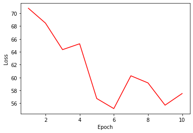
Let’s try plotting the loss curve. It can be observed that the loss drops abruptly around the fifth epoch.

# loss curve
plt.plot(range(1, NUM_EPOCHS+1), current_loss, 'r-')
plt.xlabel('Epoch')
plt.ylabel('Loss')
plt.show()

References

In this posting, we looked into implementing the Seq2Seq model by Sutskever et al. (2014). In the following postings, let’s look into the details of the Seq2Seq model with the natural extension of alignment networks.

Attention in Neural Networks - 5. Sequence-to-Sequence (Seq2Seq) (4)

|

Attention Mechanism in Neural Networks - 5. Sequence-to-Sequence (Seq2Seq) (4)

In the previous posting, we looked into implementing the Seq2Seq model by Cho et al. (2014) with Pytorch. In this posting, let’s see how we can train the model with the prepared data and evaluate it qualitatively.

Creating encoder/decoder models

First, let’s create the encoder and decoder models separately. Although they are trained and evaluated jointly, we define and create them separately for better readability and understandability of the code.

encoder = Encoder(ENG_VOCAB_SIZE, HIDDEN_SIZE, EMBEDDING_DIM).to(DEVICE)
decoder = Decoder(DEU_VOCAB_SIZE, HIDDEN_SIZE, EMBEDDING_DIM).to(DEVICE)

Just FYI, we set the hyperparameters in the previous posting as below.

  • MAX_SENT_LEN: maximum sentence length of the source (English) sentence
  • ENG_VOCAB_SIZE, DEU_VOCAB_SIZE: number of unique tokens (words) in English and German, respectively
  • NUM_EPOCHS: number of epochs to train the Seq2Seq model
  • HIDDEN_SIZE: dimensionality of the hidden space in LSTM (or any RNN variant of choice)
  • EMBEDDING_DIM: dimensionality of the word embedding space
MAX_SENT_LEN = len(max(eng_sentences, key = len))
ENG_VOCAB_SIZE = len(eng_words)
DEU_VOCAB_SIZE = len(deu_words)
NUM_EPOCHS = 1
HIDDEN_SIZE = 128
EMBEDDING_DIM = 30
DEVICE = torch.device('cuda') 

Training the dmoel

Prior to training, we create optimizers and define the loss function. The optimizers for encoder/decoder are defined similar to other deep learning models, using the Adam optimizer. We define the loss function as the negative log likelihood loss, which is one of log functions for multi-class classification. Remember that we are classifying each target word among possible unique words in German. The negative log likelihood loss can be implemented with NLLLoss() in torch.nn. For more information, please refer to documentation. Finally, traces of loss are contained in the current_loss list.

encoder_opt = torch.optim.Adam(encoder.parameters(), lr = 0.01)
decoder_opt = torch.optim.Adam(decoder.parameters(), lr = 0.01)
criterion = nn.NLLLoss()
current_loss = []

Now, we are finally ready to actually train the encoder and decoder!

  • Fetch source and target sentences and convert them into Pytorch tensors. As sentences differ in lengths, we train them one by one.
  • Initialize the hidden state (and cell state if using LSTM).
  • Train the encoder. We preserve the hidden and cell states from the last input in the source sentence and pass them onto the decoder.
  • Train the decoder. The decoder is similarly trained to the encoder, with the difference of marking the loss and terminating the loop when we encounter the end of sentence token <eos>.
for i in tqdm(range(NUM_EPOCHS)):
  for j in tqdm(range(len(eng_sentences))):
    source, target = eng_sentences[j], deu_sentences[j]
    source = torch.tensor(source, dtype = torch.long).view(-1, 1).to(DEVICE)
    target = torch.tensor(target, dtype = torch.long).view(-1, 1).to(DEVICE)

    loss = 0
    h0 = torch.zeros(1, 1, encoder.hidden_size).to(DEVICE)
    c0 = torch.zeros(1, 1, encoder.hidden_size).to(DEVICE)

    encoder_opt.zero_grad()
    decoder_opt.zero_grad()

    enc_output = torch.zeros(MAX_SENT_LEN, encoder.hidden_size)
    for k in range(source.size(0)):
      out, (h0, c0) = encoder(source[k].unsqueeze(0), h0, c0)
      enc_output[k] = out.squeeze()
    
    dec_input = torch.tensor([[deu_words.index("<sos>")]]).to(DEVICE)
    for k in range(target.size(0)):
      out, (h0, c0) = decoder(dec_input, h0, c0)
      _, max_idx = out.topk(1)
      dec_input = max_idx.squeeze().detach()
      loss += criterion(out, target[k])
      if dec_input.item() == deu_words.index("<eos>"):
        break

    loss.backward()
    encoder_opt.step()
    decoder_opt.step()
    current_loss.append(loss.item()/(j+1))

Evaluation

We can have a grasp on how the Seq2Seq model was trained by looking into each instance and its output. In this example, let’s examine the 106th instance with the words “go” and “away”. Evaluation is very similar to training, but we do it without computing the gradients and updating the weights. This can be done by the with torch.no_grad(): statement.

idx = 106   # index of the sentence that you want to demonstrate
torch.tensor(eng_sentences[idx], dtype = torch.long).view(-1, 1).to(DEVICE)
with torch.no_grad():
  h0 = torch.zeros(1, 1, encoder.hidden_size).to(DEVICE)
  c0 = torch.zeros(1, 1, encoder.hidden_size).to(DEVICE)
  enc_output = torch.zeros(MAX_SENT_LEN, encoder.hidden_size)
  for k in range(source.size(0)):
    out, (h0, c0) = encoder(source[k].unsqueeze(0), h0, c0)
    enc_output[k] = out.squeeze()
    
  dec_input = torch.tensor([[deu_words.index("<sos>")]]).to(DEVICE)
  dec_output = []
  for k in range(target.size(0)):
    out, (h0, c0) = decoder(dec_input, h0, c0)
    _, max_idx = out.topk(1)
    dec_output.append(max_idx.item())
    dec_input = max_idx.squeeze().detach()
    if dec_input.item() == deu_words.index("<eos>"):
      break

# print out the source sentence and predicted target sentence
print([eng_words[i] for i in eng_sentences[idx]])
print([deu_words[i] for i in dec_output])
['<sos>', 'go', 'away', '<eos>']
['<sos>', 'komm', 'sie', 'nicht', '<eos>']

Note that the model is poorly trained. We have sampled only 50,000 instances and trained for only one epoch without any hyperparameter tuning. You can try out various settings with expanded data in your machine. Please let me know how you improved the model!

References

In this posting, we looked into training and evaluating the Seq2Seq model with Pytorch. In the next posting, let’s look into the variants of the RNN Encoder-Decoder network proposed by Cho et al. (2014). Thank you for reading.

Attention in Neural Networks - 4. Sequence-to-Sequence (Seq2Seq) (3)

|

Attention Mechanism in Neural Networks - 4. Sequence-to-Sequence (Seq2Seq) (3)

In the previous posting, we saw how to prepare machine translation data for Seq2Seq. In this posting, let’s implement the Seq2Seq model delineated by Cho et al. (2014) with Pytorch with the prepared data.

Data Preparation

After data processing, we have four variables that contain critical information for learning a Seq2Seq model. In the previous posting, we named them eng_words, deu_words, eng_sentences, deu_sentences. eng_words and deu_words contain unique words in source (English) and target (German) sentences. In my processed data, there were 9,199 English and 16,622 German words but note that it can differ in your results since we randomly sampled 50,000 sentences.

eng_words, deu_words = list(eng_words), list(deu_words)

# print the size of the vocabulary
print(len(eng_words), len(deu_words))
9199 16622

eng_sentences and deu_sentences contain source (English) and target(German) sentences in which words are indexed according to the position in eng_words and deu_words lists. For instance, first elements in our lists were [4977, 8052, 5797, 8153, 5204, 2964, 6781, 7426] and [9231, 8867, 7020, 936, 13206, 5959, 13526]. And they correspond to English and German sentences ['<sos>', 'so', 'far', 'everything', 'is', 'all', 'right', '<eos>'] and ['<sos>', 'soweit', 'ist', 'alles', 'in', 'ordnung', '<eos>'].

print(eng_sentences[0])
print([eng_words[x] for x in eng_sentences[0]])
print(deu_sentences[0])
print([deu_words[x] for x in deu_sentences[0]])
[4977, 8052, 5797, 8153, 5204, 2964, 6781, 7426]
['<sos>', 'so', 'far', 'everything', 'is', 'all', 'right', '<eos>']
[9231, 8867, 7020, 936, 13206, 5959, 13526]
['<sos>', 'soweit', 'ist', 'alles', 'in', 'ordnung', '<eos>']

Parameter setting

Now, let’s move onto setting hyperparameters for our Seq2Seq model. Key parameters and their descriptions are as below.

  • MAX_SENT_LEN: maximum sentence length of the source (English) sentence
  • ENG_VOCAB_SIZE, DEU_VOCAB_SIZE: number of unique tokens (words) in English and German, respectively
  • NUM_EPOCHS: number of epochs to train the Seq2Seq model
  • HIDDEN_SIZE: dimensionality of the hidden space in LSTM (or any RNN variant of choice)
  • EMBEDDING_DIM: dimensionality of the word embedding space

We set the parameters as below. Note that NUM_EPOCHS, HIDDEN_SIZE, and EMBEDDING_DIM variables can be arbitrarily set by the user as in any other neural network architecture. You are strongly encouraged to test other parameter settings and compare the results.

MAX_SENT_LEN = len(max(eng_sentences, key = len))
ENG_VOCAB_SIZE = len(eng_words)
DEU_VOCAB_SIZE = len(deu_words)
NUM_EPOCHS = 1
HIDDEN_SIZE = 128
EMBEDDING_DIM = 30
DEVICE = torch.device('cuda') 

RNN in Pytorch

Prior to implemeting the encoder and decoder, let’s briefly review the inner workings of RNNr and how they are implemented in Pytorch. We will implement the Long Short-Term Memory (LSTM), which is a popular variant of RNN.

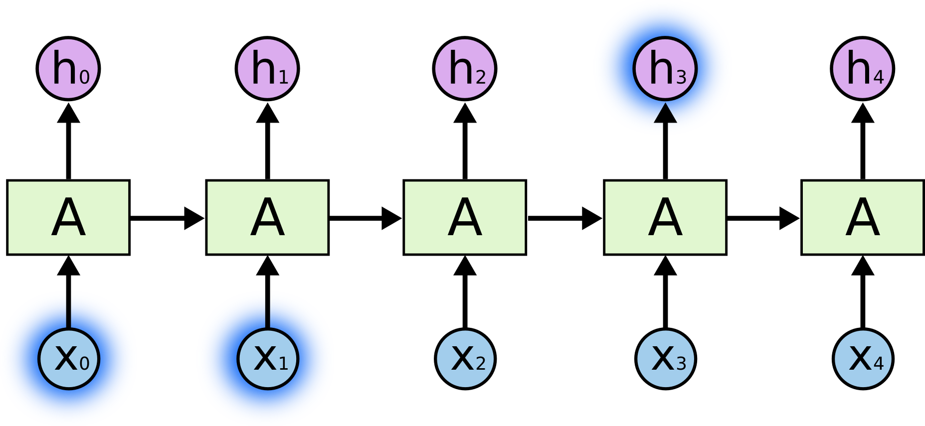
[Image source]

RNNs in general are used for modeling temporal dependencies among inputs in consecutive timesteps. Unlike feed-forward neural networks, they have “loops” in the network, letting the information flow between timesteps. Such information is stored and passed onto as “hidden states.” For each input (\(x_i\)), there is a corresponding hidden state (\(h_i\)) that preserves information at that time step \(i\). And that hidden state is also an input at the next time step with \(x_{i+1}\). At the first timestemp (0), they are randomly initialized.

In addition to the hidden state, there is additional information that is passed onto the next state, namely the cell state (\(c_i\)). The math behind it is complicated but I won’t be going into detail . For the sake of simplicity, we can regard it as another type of hidden state in this posting. For more information, please refer to Hochreiter et al. (1997).

Once we understand the inner workings of RNN, it is fairly straightforward to implement it with Pytorch.

import torch.nn as nn
lstm = nn.LSTM(input_size = 10, 
             hidden_size = 5, 
             num_layers = 1)
  • Create LSTM layer: there are a few parameters to be determined. Some of the essential ones are input_size, hidden_size, and num_layers. input_size can be regarded as a number of features. Each input in each timestemp is an n-dimensional vector with n = input_size. hidden_size is the dimensionality of the hidden state. Each hidden state is an m-dimensional vector with m = hidden_size. Finally num_layers determines the number of layers in the LSTM layer. Setting it over 3 makes it a deep LSTM.
## inputs to LSTM
# input data (seq_len, batch_size, input_size)
x0 = torch.from_numpy(np.random.randn(1, 64, 10)).float()     
  • Determine input size: The shape of inputs to the LSTM layer is (seq_len, batch_size, input_size). seq_len determines the length of the sequence, or the number of timesteps. In the machine translation task, this should be the number of source (or target) words in the instance. input_size should be the same as one defined when creating the LSTM layer.
h0, c0 = torch.from_numpy(np.zeros((1, 64, 5))).float(), torch.from_numpy(np.zeros((1, 64, 5))).float()
  • Initialize hidden & cell states: hidden and cell states have the same shape (num_layers, batch_size, hidden_size) in general. Note that we need not consider seq_len since hidden and cell states are refreshed at each time step.
xn, (hn, cn) = lstm(x0, (h0, c0))

print(xn.shape)               # (seq_len, batch_size, hidden_size)
print(hn.shape, cn.shape)     # (num_layers, batch_size, hidden_size)
torch.Size([1, 64, 5])
torch.Size([1, 64, 5]) torch.Size([1, 64, 5])
  • Pass the input and hidden/cell states to LSTM: Now we just need to pass the input and states to the LSTM layer. Note that the hidden and cell states are provided in a single tuple (h0, c0). The output sizes are identical to the inputs.

If you want to learn more about RNNs in Pytorch, please refer to Pytorch Tutorial on RNN.

Encoder

Now, we have to construct the neural network architecture for Seq2Seq. Here, we construct the encoder and decoder network separately since it can be better understood that way.

Encoder is a relatively simple neural network consisting of embedding and RNN layers. We inject each word in the source sentence (English words in this case) to LSTM after embedding. Note that we have to set three parameters for the encoder network - vocab_size, hidden_size, and embedding_dim. They will correspond to ENG_VOCAB_SIZE, HIDDEN_SIZE, and EMBEDDING_DIM variables defined above.

class Encoder(nn.Module):
  def __init__(self, vocab_size, hidden_size, embedding_dim):
    super(Encoder, self).__init__()
    self.hidden_size = hidden_size

    self.embedding = nn.Embedding(vocab_size, embedding_dim)
    self.lstm = nn.LSTM(embedding_dim, hidden_size)

  def forward(self, x, h0, c0):
    x = self.embedding(x).view(1, 1, -1)
    out, (h0, c0) = self.lstm(x, (h0, c0))
    return out, (h0, c0)

The “hidden state” (h0) from the final source word will be memorized and passed onto the decoder as an input. This is a fixed-sized vector “summary c of the whole input sequence.”

Decoder

Finally, we will have to define the decoder network. The decoder is very similar to the encoder with a slight difference. Other information except the hidden state is discarded in the encoder network. In other words, all information from the input sentence is summarized in the hidden state. Nevertheless, in the decoder, a previous (predicted) word should be passed onto the next LSTM cell for the next prediction. Therefore, we generate another dense layer followed by a softmax activation function to track the predicted word and pass them onto the next step.

class Decoder(nn.Module):
  def __init__(self, vocab_size, hidden_size, embedding_dim):
    super(Decoder, self).__init__()
    self.hidden_size = hidden_size

    self.embedding = nn.Embedding(vocab_size, embedding_dim)
    self.lstm = nn.LSTM(embedding_dim, hidden_size)
    self.dense = nn.Linear(hidden_size, vocab_size)
    self.softmax = nn.LogSoftmax(dim = 1)
  
  def forward(self, x, h0, c0):
    x = self.embedding(x).view(1, 1, -1)
    x, (h0, c0) = self.lstm(x, (h0, c0))
    x = self.softmax(self.dense(x.squeeze(0)))
    return x, (h0, c0)

As we defined classes to generate the encoder and decoder, we now just have to create and train them!

References

In this posting, we implemented the Seq2Seq model with Pytorch. In the next posting, let’s look into how we can train and evaluate them with the prepared data. Thank you for reading.