Attention Mechanism in Neural Networks - 3. Sequence-to-Sequence (Seq2Seq) (2)

In the previous posting, we had a first look into Sequence-to-Sequence (Seq2Seq). In this posting, prior to implementing Seq2Seq models with Python, let’s see how to prepare data for neural machine translation.

Problem - neural machine translation

The task of machine translation is to automate the process of converting sentences in one language (e.g., French) to ones in another language (e.g., English). The sentences (words) that we want to convert are often called source sentences (words). And sentences (words) that are converted into are target sentences (words). In the diagram below demonstrating translation from French to English, the first source words are “On”, “y” and “va,” while target words are “Let’s” and “go.”

Neural machine translation is a branch of machine translation that actively utilizes neural networks, such as recurrent neural networks and multilayer perceptrons, to predict the likelihood of a possible word sequence in the corpus. So far, neural machine translation has more succesfully tackled problems in machine translation that have outlined in the previous posting.

Many of earlier ground-breaking studies in neural machine translation employ Seq2Seq architecture, e.g., Cho et al. (2014). In this posting, let’s look into how to prepare data for neural machine translation with Python. I will use Google Colaboratory for this attention posting series, so if you are new to it, please check out my posting on Colaboratory.

[Image source: Cho et al. (2014)]

Dataset

The dataset used in this posting is English-German sentence pairs dataset downloaded from here. They provide not only German sentences corresponding to English ones, but also other languages such as French, Arabic, and Chinese. So if you want to try out translating other languages, please check out the website!

[Image source]

The data are tab-separated, with each line consisting of English sentence + TAB + Another language sentence + TAB + Attribution. Therefore, we can extract (English sentence, another language sentence) from each line while splitting each line with TAB (“\t”).

[Image source]

Let’s start out with importing necessary packages. We do not need many packages for this practice and they are already installed in the Colab environment. We just need to import them.

import re
import torch
import numpy as np
import torch.nn as nn
from tqdm import tqdm

Download & Read data

Let’s download and unzip the dataset first. You can also manually download and unzip them in your machine, but you can just run below Linux command in your colaboratory file.

!wget https://www.manythings.org/anki/deu-eng.zip
!unzip deu-eng.zip

You will get below output if the file is successfully downloaded and unzipped.

-2020-01-13 09:30:06--  https://www.manythings.org/anki/deu-eng.zip
Resolving www.manythings.org (www.manythings.org)... 104.24.108.196, 104.24.109.196, 2606:4700:30::6818:6dc4, ...
Connecting to www.manythings.org (www.manythings.org)|104.24.108.196|:443... connected.
HTTP request sent, awaiting response... 200 OK
Length: 7747747 (7.4M) [application/zip]
Saving to: ‘deu-eng.zip’

deu-eng.zip         100%[===================>]   7.39M  7.53MB/s    in 1.0s    

2020-01-13 09:30:13 (7.53 MB/s) - ‘deu-eng.zip’ saved [7747747/7747747]

Archive:  deu-eng.zip
  inflating: deu.txt                 
  inflating: _about.txt  

After the file is downloaded, we can open the file and read them. I prefer to read txt files with the readlines() function, but you can also try it with the read() function.

with open("deu.txt") as f:
  sentences = f.readlines()
 # number of sentences
len(sentences)

The length of the list storing data is 200,519. In other words, there are 200,519 English-German sentence pairs in total.

200519

Preprocessing

Every dataset needs preprocessing, especially it is unstructured data like text. For the sake of minimizing time and computational costs involved, we will randomly choose 50,000 pairs for training the model. Then, we will leave only alphabetic characters and tokenize the sentence. Also, letters will be changed into lowercase letters and unique tokens will be extracted in separate sets. In addition, we add “start of the sentence” ("<sos>") and “end of the sentence” (<eos>) tokens to the start and end of the sentences. This will let the machine detect the head and tail of each sentence.

NUM_INSTANCES = 50000
eng_sentences, deu_sentences = [], []
eng_words, deu_words = set(), set()
for i in tqdm(range(NUM_INSTANCES)):
  rand_idx = np.random.randint(len(sentences))
  # find only letters in sentences
  eng_sent, deu_sent = ["<sos>"], ["<sos>"]
  eng_sent += re.findall(r"\w+", sentences[rand_idx].split("\t")[0]) 
  deu_sent += re.findall(r"\w+", sentences[rand_idx].split("\t")[1])

  # change to lowercase
  eng_sent = [x.lower() for x in eng_sent]
  deu_sent = [x.lower() for x in deu_sent]
  eng_sent.append("<eos>")
  deu_sent.append("<eos>")

  # add parsed sentences
  eng_sentences.append(eng_sent)
  deu_sentences.append(deu_sent)

  # update unique words
  eng_words.update(eng_sent)
  deu_words.update(deu_sent)

So, now we have 50,000 randomly selected English and German sentences that are paired with corresponding indices. To get the indices for the tokens, let’s convert the unique token sets into lists. Then, for the sanity check, let’s print out the sizes of the English and German vocabulary in the corpus.

eng_words, deu_words = list(eng_words), list(deu_words)

# print the size of the vocabulary
print(len(eng_words), len(deu_words))

There are 9,209 unqiue English tokens and 16,548 German tokens. It is interesting to see there are about two times more tokens in German than in English.

9209 16548

Finally, let’s convert words in each sentence into indices. This will make the information more accessible and understandable for the machine. Such indexed sentences will be inputs for the implemented neural network models.

# encode each token into index
for i in tqdm(range(len(eng_sentences))):
  eng_sentences[i] = [eng_words.index(x) for x in eng_sentences[i]]
  deu_sentences[i] = [deu_words.index(x) for x in deu_sentences[i]]

Now, we are done with importing and preprocessing English-German data. For the final sanity check, let’s try printing out the encoded and raw sentences. Note that the selected sentences can be different on your side since we randomly select 50,000 sentences from the corpus.

print(eng_sentences[0])
print([eng_words[x] for x in eng_sentences[0]])
print(deu_sentences[0])
print([deu_words[x] for x in deu_sentences[0]])

[4977, 8052, 5797, 8153, 5204, 2964, 6781, 7426]
['<sos>', 'so', 'far', 'everything', 'is', 'all', 'right', '<eos>']
[9231, 8867, 7020, 936, 13206, 5959, 13526]
['<sos>', 'soweit', 'ist', 'alles', 'in', 'ordnung', '<eos>']

In this posting, Seq2Seq and its overall architecture have been introduced. In the next posting, I will implement the Seq2Seq model with Pytorch and show how to train it with the preprocessed data. Thank you for reading.

Attention Mechanism in Neural Networks - 2. Sequence-to-Sequence (Seq2Seq) (1)

In previous posting, I introduced the attention mechanism and outlined its (not so) short history. In this posting, I will explain the Sequence-to-Sequence (Seq2Seq) architecture, which brought a major breakthrough in neural machine translation and motivated the development of attention.

[Image source]

Motivation - Problem of sequences

Deep neural networks are highly effective tools to model non-linear data for various tasks. It has been proven to be effective in various tasks, e.g., image classification and sentence classification. However, conventional architectures such as multilayer perceptrons are less effective in modeling sequences such as signals and natural language. Therefore, Seq2Seq was proposed to map sequence inputs to sequence outputs. Seq2Seq can process variable-length vectors, mapping them to variable-length vectors.

[Photo by Bret Kavanaugh on Unsplash]

Consider the classical application of Seq2Seq to the machine translation task, i.e., translating French sentences (source) to English ones (target). Notice that source sentences have different lengths in terms of words (or characters). The first French sentence “On y va,” which is translated into “Let’s go” in English, has three words or the second, third, and fourth sentences have four, five, and six, respectively. Also, the number of target words are not fixed as well - it can be two to six words in this example.

Another potential problem of machine translation is that source (and target) words are often dependent on each other. For instance, when we see the word “I” at the start of the sentence, we are more likely to see “am” as the second word than “are.” Conversely, if we see “You,” we are likely to see “are” than “am.” Thus, it is important to model temporal dependencies among different words (and characters) in a sentence.

Also, source and target words have dependencies between them. In other words, a source word is more likely to be related with some of the target words than others. For instance, “Pour” in the second French sentence is more aligned with “For” in the English sentence and “la” with “the” and so on. This is more deeply considered in Alignment models with attention

Seq2Seq architecture

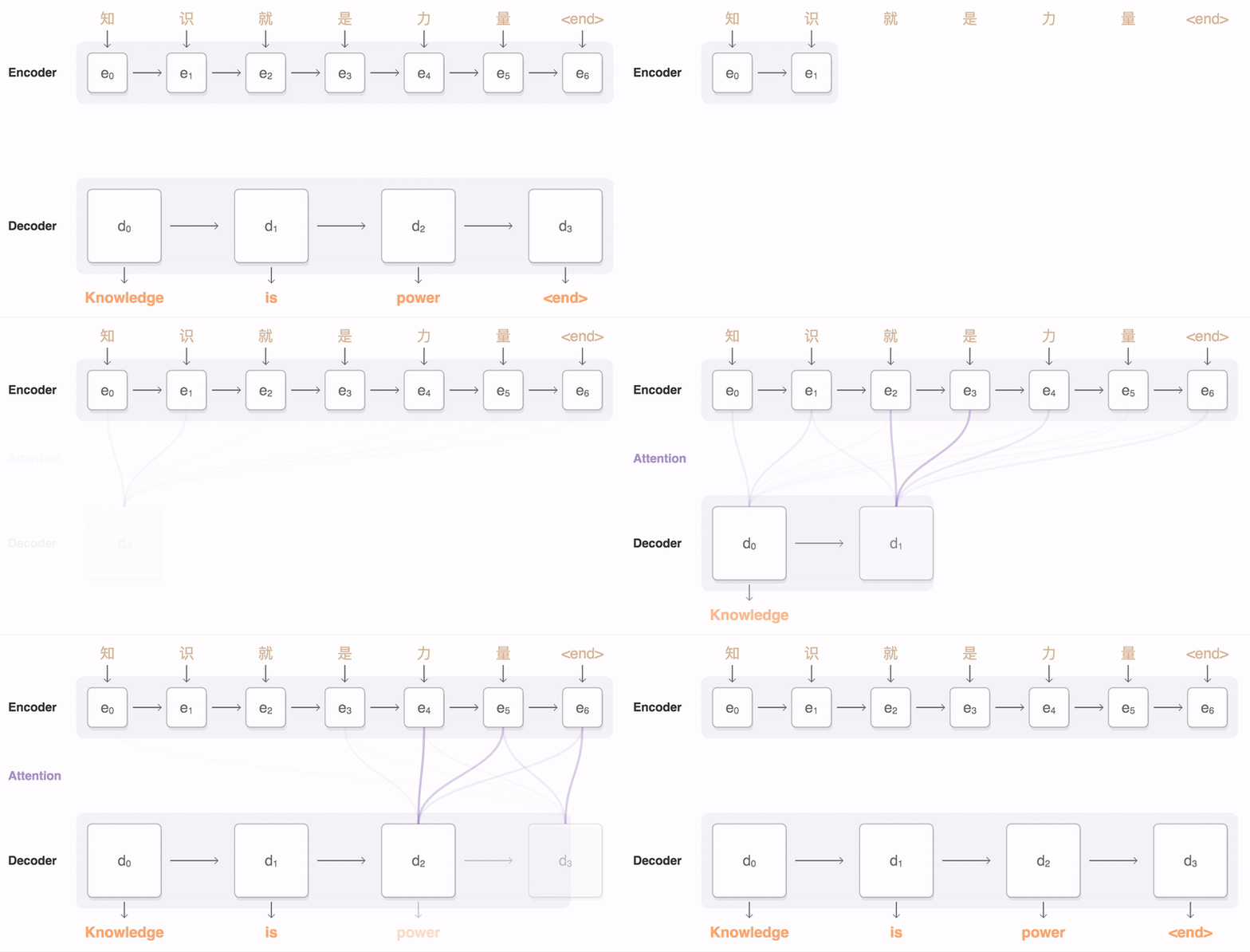
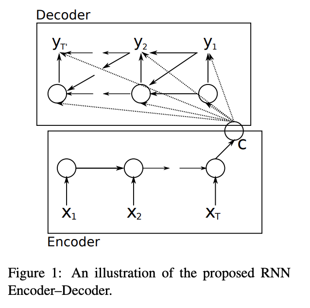
Therefore, Seq2Seq was proposed to model variable-length source inputs with temporal dependencies. Cho et al. (2014) is one of the frontier studies investigating neural machine translation with sequences. Their RNN Encoder-Decoder architecture is comprised of two recurrent neural networks - i.e., encoder and decoder.

[Image source: Cho et al. (2014)]

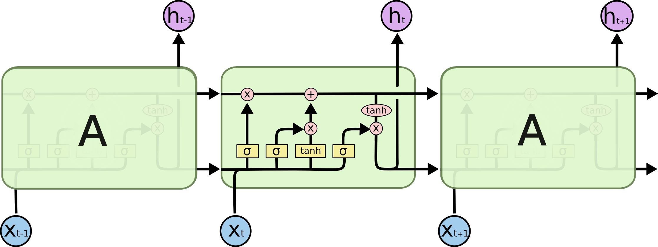
Both encoder and decoder comprise multiple recurrent neural network (RNN) cells such as LSTM and GRU cells. The number of cells varies across different instances to take into account varying number of source and target words. Each RNN cells have multiple outputs to model dependencies among input vectors. In addition to sequence outputs, LSTM cells have hidden and cell states and GRU cells have hidden states. For more information on RNN structure, please refer to RNN tutorial with Pytorch.

[Image source]

The final hidden state of the encoder, c, functions as a summary of the inputs to the encoder, i.e., the source sentence. In other words, information from the source sentence is distilled in a vector with a fixed dimensionality. In the decoder , c is an input to RNN cells, along with previous hidden state and target word. Therefore, the hidden state at level t is calculated as below (f is the RNN operation in this context).

\begin{equation} h_t = f(h_{t-1}, y_{t-1}, c) \end{equation}

And the output at each step t is the probability of predicting a certain word at that step with the activation function g.

\begin{equation} P(y_t|y_{t-1}, y_{t-2}, …, y_1, c) = g(h_t, y_{t-1}, c) \end{equation}

Then, the calculated probabilities are softmaxed to find the word with the highest predicted probability.

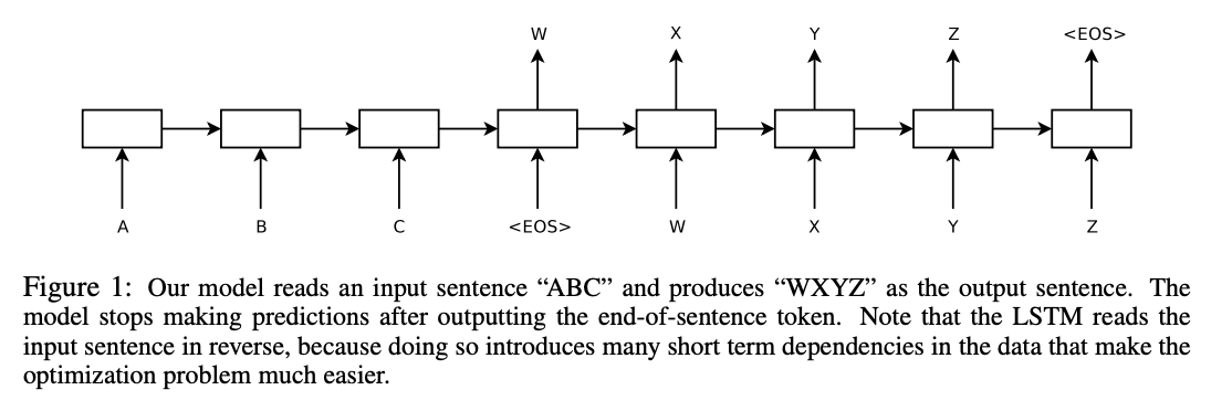
[Image source: Sutskever et al. (2014)]

Following Cho et al. (2014), many studies such as Sutskever et al. (2014) proposed similar deep learning architectures to RNN Encoder-Decoder with LSTM. Hence, we call variants of RNN models mapping sequences to sequences with the encoder and decoder Seq2Seq.

In this posting, I introduced Seq2Seq and its overall architecture. In the next posting, I will explain the Seq2Seq architecture in detail, while implementing it with Pytorch. Thank you for reading.

References

• Cho et al. (2014)
• Sutskever et al. (2014)

Updated 11/15/2020: Visual Transformer

Attention Mechanism in Neural Networks - 1. Introduction

Attention is arguably one of the most powerful concepts in the deep learning field nowadays. It is based on a common-sensical intuition that we “attend to” a certain part when processing a large amount of information.

[Photo by Romain Vignes on Unsplash]

This simple yet powerful concept has revolutionized the field, bringing out many breakthroughs in not only natural language processing (NLP) tasks, but also recommendation, healthcare analytics, image processing, speech recognition, etc.

Therefore, in this posting series, I will illustrate the development of the attention mechanism in neural networks with emphasis on applications and real-world deployment. I will try to implement as many attention networks as possible with Pytorch from scratch - from data import and processing to model evaluation and interpretations.

Final disclaimer is that I am not an expert or authority on attention. The primary purpose of this posting series is for my own education and organization. However, I am sharing my learning process here to help anyone who is eager to learn new things, just like myself. Please do not heistate leave a comment if you detect any mistakes or errors that I make, or you have any other (great) ideas and suggestions. Thank you for reading my article.

Key developments in attention

Attention mechanism was first proposed in the NLP field and still actively researched in the field. Above is the key designs and seminal papers that led to major developments. Here, I will briefly review them one by one.

• Seq2Seq, or RNN Encoder-Decoder (Cho et al. (2014), Sutskever et al. (2014))
• Alignment models (Bahdanau et al. (2015), Luong et al. (2015))
• Visual attention (Xu et al. (2015))
• Hierarchical attention (Yang et al. (2016))
• Transformer (Vaswani et al. (2017))

Sequence to sequence (Seq2Seq) architecture for machine translation

Many text information is in a sequence format, e.g., words, sentences, and documents. Seq2Seq is a two-part deep learning architecture to map sequence inputs into sequence outputs. It was initially proposed for the machine translation task, but can be applied for other sequence-to-sequence mapping tasks such as captioning and question retrieval.

Cho et al. (2014) and Sutskever et al. (2014) indepedently proposed similar deep learning architectures comprising two recurrent neural networks (RNN), namely encoder and decoder.

[Image source: Sutskever et al. (2014)]

The encoder reads a sequence input with variable lengths, e.g., English words, and the decoder produces a sequence output, e.g., corresponding French words, considering the hidden state from the encoder. The hidden state sends source information from the encoder to the decoder, linking the two. Both the encoder and decoder consist of RNN cells or its variants such as LSTM and GRU.

Align & Translate

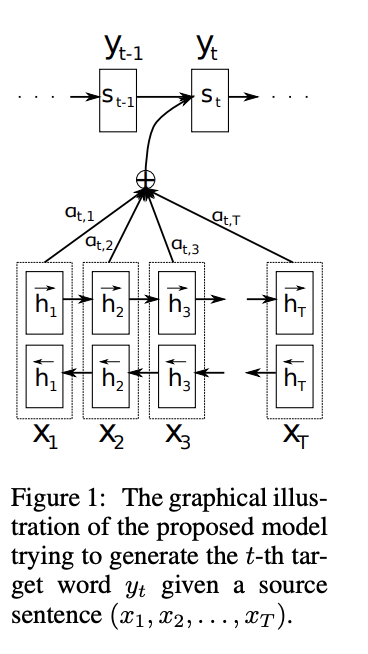
A potential problem of the vanilla Seq2Seq architecture is that some information might not be captured by a fixed-length vector, i.e., the final hidden state from the encoder ($h_t$). This can be especially problematic when processing long sentences where RNN is unable to send adequate information to the end of the sentences due to gradient exploding, etc.

[Image source: Bahdanau et al. (2015)]

Therefore, Bahdanau et al. (2015) proposed utilizing a context vector to align the source and target inputs. The context vector preserves information from all hidden states from encoder cells and aligns them with the current target output. By doing so, the model is able to “attend to” a certain part of the source inputs and learn the complex relationship between the source and target better. Luong et al. (2015) outlines various types of attention models to align the source and target.

Visual attention

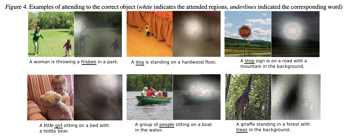
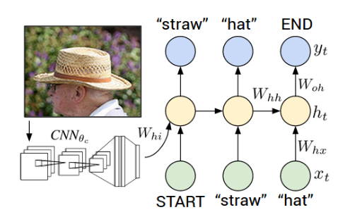
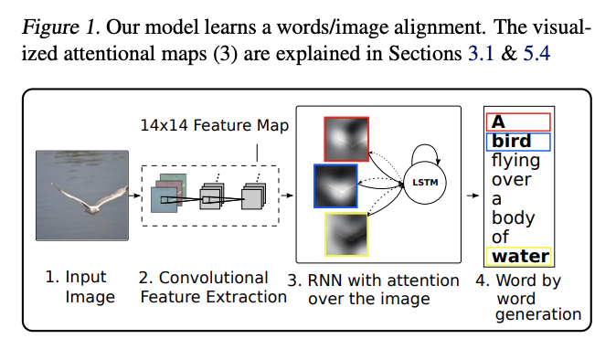
Xu et al. (2015) proposed an attention framework that extends beyond the conventional Seq2Seq architecture. Their framework attempts to align the input image and output word, tackling the image captioning problem.

[Image source: Xu et al. (2015)]

Accordingly, they utilized a convolutional layer to extract features from the image and align such features using RNN with attention. The generated words (captions) are aligned with specific parts of the image, highlighting the relevant objects as below. Their framework is one of the earlier attempts to apply attention to other problems than neural machine translation.

[Image source: Xu et al. (2015)]

Hierarchical attention

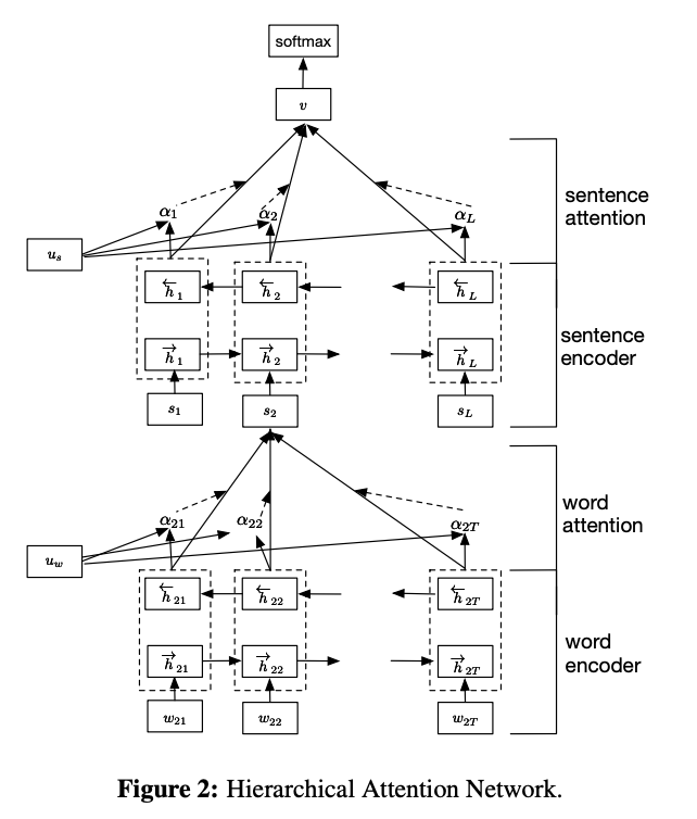
Yang et al. (2016) demonstrated with their hierarchical attention network (HAN) that attention can be effectively used on various levels. Also, they showed that attention mechanism applicable to the classification problem, not just sequence generation.

[Image source: Yang et al. (2016)]

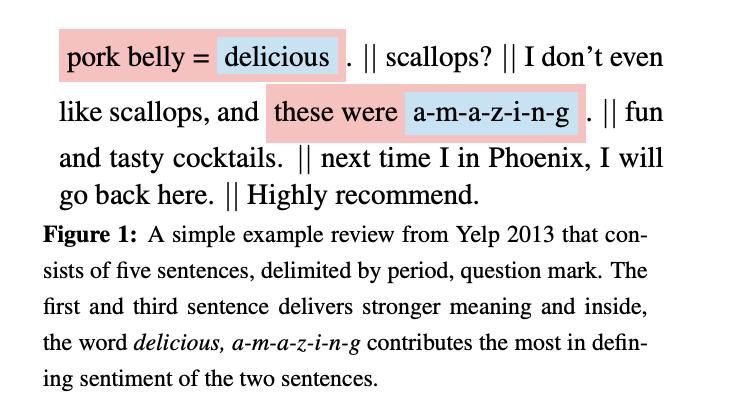
HAN comprises two encoder networks - i.e., word and sentence encoders. The word encoder processes each word and aligns them a sentence of interest. Then, the sentence encoder aligns each sentence with the final output. HAN enables hierarchical interpretation of results as below. The user can understand (1) which sentence is crucial in classifying the document and (2) which part of the sentence, i.e., which words, are salient in that sentence.

[Image source: Yang et al. (2016)]

Transformer and BERT

[Image source: Vaswani et al. (2017)]

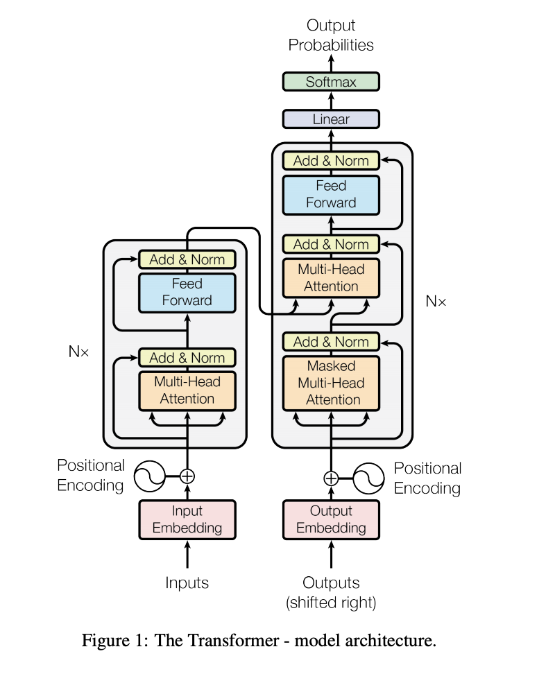
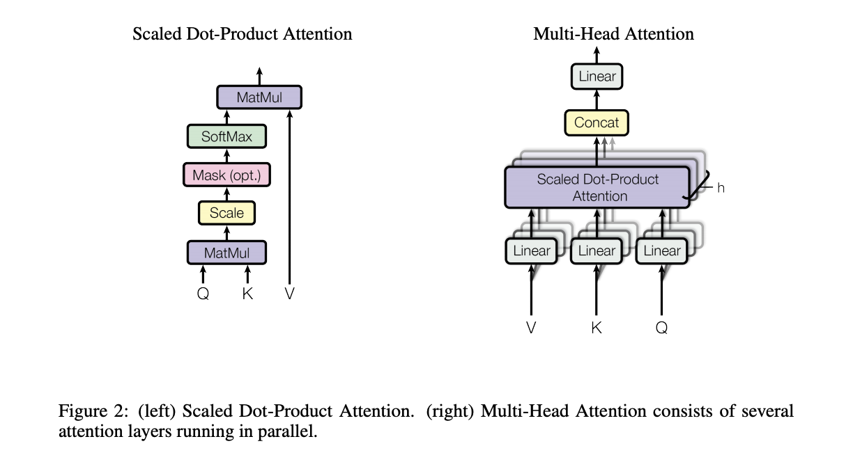
The Transformer neural network architecture proposed by Vaswani et al. (2017) marked one of the major breakthroughs of the decade in the NLP field. The multi-head self-attention layer in Transformer aligns words in a sequence with other words in the sequence, thereby calculating a representation of the sequence. It is not only more effective in representation, but also more computationally efficient compared to convolution and recursive operations.

[Image source: Vaswani et al. (2017)]

Thus, the Transformer architecture discards the convolution and recursive operations and replaces them with multi-head attention. The multi-head attention is essentially multiple attention layers jointly learning different representations from different positions.

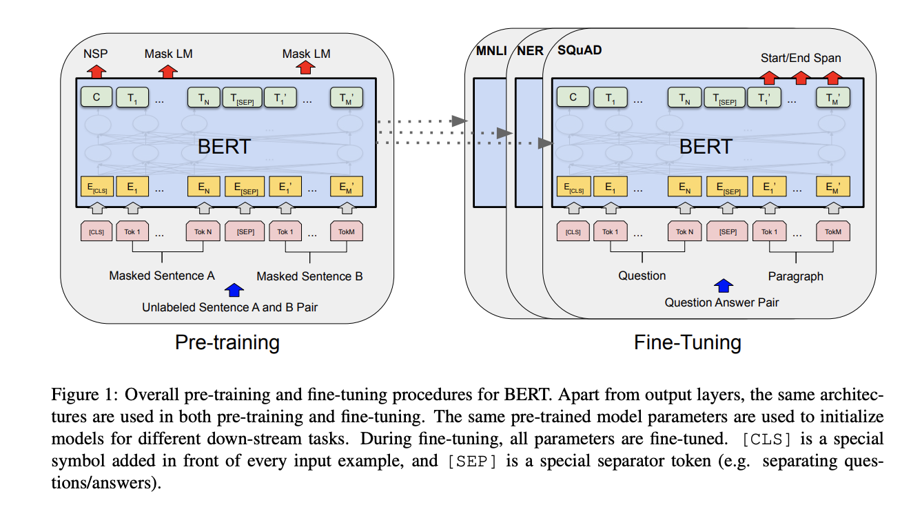
[Image source: Devlin et al. (2018)]

The intuition behind Transformer inspired a number of researchers, leading to the development of self-attention-based models such as Bidirectional Encoder Representations from Transformers (BERT) by Devlin et al. (2019). BERT pretrains bidirectional representations with the improved Transformer architecture. BERT shows state-of-the-art performance in various NLP tasks as of 2019. And there have a number of transformer-based language models that showed breakthrough results such as XLNet, RoBERTa, GPT-2, and ALBERT.

Vision Transformer

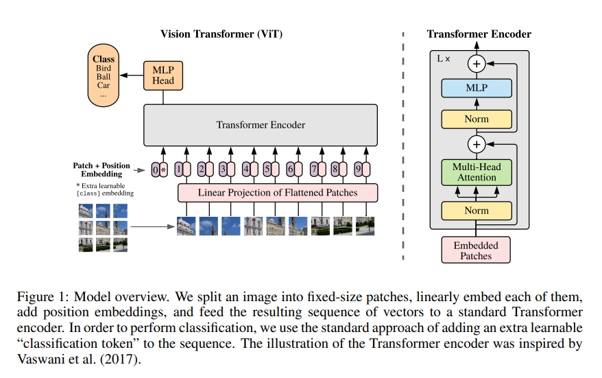
In the last few years, Transformer definitely revolutionalized the NLP field. Transformer-inspired models such as GPT and BERT showed record-breaking results on numerous NLP tasks. With that said, Dosovitskiy et al. (2020) demonstrated claimed that Transformer can be used for computer vision tasks, which is another AI-complete problem. This might sound a bit outdated since attention has been used for image-related tasks fairly extensively, e.g., Xu et al. (2015).

However, Dosovitskiy et al. (2020)’s claim is revolutionary since in their proposed model architecture, Transformer virtually replaces convolutional layers rather than complementing them. Furthermore, the Vision Transformer outperforms state-of-the-art, large-scale CNN models when trained with sufficient data. This might mean that CNN’s golden age, which lasted for years, can come to end similar to that of RNN by Transformer.

[Image source: Dosovitskiy et al. (2020) ]

Other applications

I have outlined major developments in attention with emphasis on NLP in this posting. However, attention mechanism is now widely used in a number of applications as mentioned. Below are some examples of successful applications of attention in other domains. However, attention mechanism is very actively researched nowadays and it is expected that there will be (is) more and more domains welcoming the application of attentional models.

• Heathcare: Choi et al. (2016)
• Speech recognition: Chorowski et al. (2015)
• Graph attention networks: Velickovic´ et al. (2018)
• Recommender systems: Seo et al. (2017) Tay et al. (2018)
• Self-driving cars: Kim and Canny (2017)

In this posting, the concept of attention mechanism was gently introduced and major developments so far were outlined. From the next posting, we will look into details of key designs of seminal models. Let’s start out with the Seq2Seq model that motivated the development of alignment models.

References

• Cho et al. (2014)
• Sutskever et al. (2014)
• Bahdanau et al. (2015)
• Luong et al. (2015)
• Xu et al. (2015)
• Yang et al. 2016
• Vaswani et al. (2017)
• Devlin et al. (2019)
• Dosovitskiy et al. (2020)

Videos for more intuitive and in-depth explanations on attention…

• Attention and Memory in Deep Learning (DeepMind)
• Neural Machine Translation and Models with Attention (Chris Manning)
• Attention Model (Andrew Ng)

Links to this posting series

• Seq2Seq (1) - Introduction to Seq2Seq
• Seq2Seq (2) - Preparing data for machine translation Seq2Seq / Colab Notebook
• Seq2Seq (3) - Implementation of Seq2Seq / Colab Notebook
• Seq2Seq (4) - Training and evaluating Seq2Seq / Colab Notebook
• Seq2Seq (5) - Variant of Seq2Seq / Colab Notebook
• Seq2Seq (6) - Mini-batch Seq2Seq / Colab Notebook

순환형 신경망 8 - CuDNNGRU & CuDNNLSTM

Objective: 케라스로 CuDNNLSTM과 CuDNNGRU 모델을 구현해 본다

이번 포스팅에서는 GPU를 활용하여 기존의 LSTM/GRU보다 더 빠르게 학습할 수 있는 CuDNNLSTM과 CuDNNGRU를 구현해 보자.

데이터 셋 불러오기

CNN-RNN 모델을 학습하기 위한 IMDB 데이터 셋을 불러온다.

num_words = 30000
maxlen = 300

(X_train, y_train), (X_test, y_test) = imdb.load_data(num_words = num_words)

# pad the sequences with zeros 
# padding parameter is set to 'post' => 0's are appended to end of sequences
X_train = pad_sequences(X_train, maxlen = maxlen, padding = 'post')
X_test = pad_sequences(X_test, maxlen = maxlen, padding = 'post')

X_train = X_train.reshape(X_train.shape + (1,))
X_test = X_test.reshape(X_test.shape + (1,))

print(X_train.shape)
print(X_test.shape)
print(y_train.shape)
print(y_test.shape)

(25000, 300, 1)
(25000, 300, 1)
(25000,)
(25000,)

LSTM

CuDNN을 활용하지 않은 기존의 LSTM

def lstm_model():
    model = Sequential()
    model.add(LSTM(50, input_shape = (300,1), return_sequences = True))
    model.add(LSTM(1, return_sequences = False))
    model.add(Activation('sigmoid'))
    
    model.compile(loss = 'binary_crossentropy', optimizer = 'adam', metrics = ['accuracy'])
    return model

 model = lstm_model()

 %%time
model.fit(X_train, y_train, batch_size = 100, epochs = 10, verbose = 0)

Wall time: 29min 40s

기존의 LSTM 모델은 epoch 10회를 학습하는 데 30분 가량 걸리는 것을 볼 수 있다.

GRU

CuDNN을 활용하지 않은 기존의 GRU

def gru_model():
    model = Sequential()
    model.add(GRU(50, input_shape = (300,1), return_sequences = True))
    model.add(GRU(1, return_sequences = False))
    model.add(Activation('sigmoid'))
    
    model.compile(loss = 'binary_crossentropy', optimizer = 'adam', metrics = ['accuracy'])
    return model

model = gru_model()
%%time
model.fit(X_train, y_train, batch_size = 100, epochs = 10, verbose = 0)

Wall time: 21min 46s

기존의 GRU 모델은 학습에 있어 20분 정도 걸리는 것을 볼 수 있다. GRU가 LSTM에 비해 셀 구조가 단순해 LSTM에 비해서 적은 학습 시간을 필요로 한다.

CuDNN LSTM

CuDNN을 활용한 CuDNNLSTM

def cudnn_lstm_model():
    model = Sequential()
    model.add(CuDNNLSTM(50, input_shape = (300,1), return_sequences = True))
    model.add(CuDNNLSTM(1, return_sequences = False))
    model.add(Activation('sigmoid'))
    
    model.compile(loss = 'binary_crossentropy', optimizer = 'adam', metrics = ['accuracy'])
    return model

model = cudnn_lstm_model()

%%time
model.fit(X_train, y_train, batch_size = 100, epochs = 10, verbose = 0)

Wall time: 2min 53s

CuDNN LSTM은 3분 이내의 학습 시간을 보이며 기존의 LSTM에 비해 10배 가량 빠른 학습 속도를 보여준다.

CuDNN GRU

CuDNN을 활용한 GRU

def cudnn_gru_model():
    model = Sequential()
    model.add(CuDNNGRU(50, input_shape = (300,1), return_sequences = True))
    model.add(CuDNNGRU(1, return_sequences = False))
    model.add(Activation('sigmoid'))
    
    model.compile(loss = 'binary_crossentropy', optimizer = 'adam', metrics = ['accuracy'])
    return model

model = cudnn_gru_model()

%%time
model.fit(X_train, y_train, batch_size = 100, epochs = 10, verbose = 0)

Wall time: 1min 54s

CuDNN GRU도 역시 기존의 GRU에 비해 10배 가량 빠른 학습 속도를 보여준다.

전체 코드

본 실습의 전체 코드는 여기에서 열람하실 수 있습니다!

순환형 신경망 7 - CNN-RNN 모델

Objective: 케라스로 RNN 모델을 구현해 본다

이번 포스팅에서는 서로 다른 형태의 인공신경망 구조인 CNN과 RNN을 합성한 CNN-RNN 모델을 구현하고 학습해 보자.

데이터 셋 불러오기

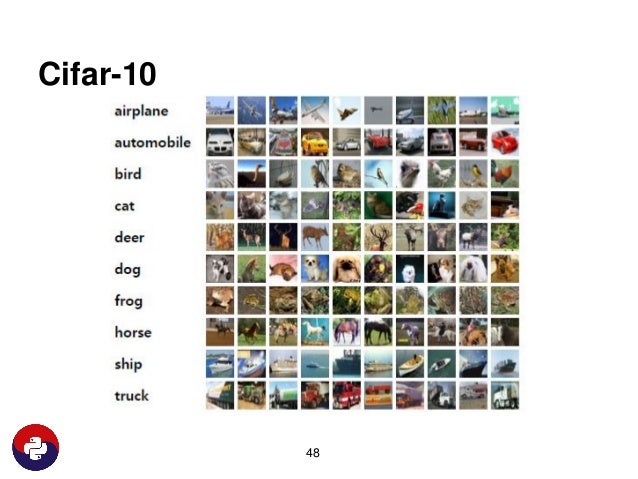
CNN-RNN 모델을 학습하기 위한 CIFAR-10 데이터 셋을 불러온다.

• source: https://www.cs.toronto.edu/~kriz/cifar.html

import numpy as np

from sklearn.metrics import accuracy_score
from keras.datasets import cifar10
from keras.utils import to_categorical

(X_train, y_train), (X_test, y_test) = cifar10.load_data()

y_train = to_categorical(y_train)
y_test = to_categorical(y_test)

print(X_train.shape)
print(X_test.shape)
print(y_train.shape)
print(y_test.shape)

(50000, 32, 32, 3)
(10000, 32, 32, 3)
(50000, 10)
(10000, 10)

CNN-RNN

• Convolution과 pooling 연산을 순차적으로 수행한 후 그 결과를 RNN 구조로 이어 학습한다.
• 이미지 캡셔닝(이미지 설명)에 활용되는 모형과 비슷한 구조라고 할 수 있다

from keras.models import Sequential, Model
from keras.layers import Conv2D, MaxPooling2D, Flatten, Dense, LSTM, Input, Activation, Reshape, concatenate
from keras import optimizers

model = Sequential()

model.add(Conv2D(input_shape = (X_train.shape[1], X_train.shape[2], X_train.shape[3]), filters = 50, kernel_size = (3,3), strides = (1,1), padding = 'same'))
model.add(Activation('relu'))
model.add(MaxPooling2D(pool_size = (2,2)))

model.add(Reshape(target_shape = (16*16, 50)))
model.add(LSTM(50, return_sequences = False))

model.add(Dense(10))
model.add(Activation('softmax'))
adam = optimizers.Adam(lr = 0.001)
model.compile(loss = 'categorical_crossentropy', optimizer = adam, metrics = ['accuracy'])

print(model.summary())

Layer (type)                 Output Shape              Param #   
=================================================================
conv2d_8 (Conv2D)            (None, 32, 32, 50)        1400      
_________________________________________________________________
activation_18 (Activation)   (None, 32, 32, 50)        0         
_________________________________________________________________
max_pooling2d_7 (MaxPooling2 (None, 16, 16, 50)        0         
_________________________________________________________________
reshape_6 (Reshape)          (None, 256, 50)           0         
_________________________________________________________________
lstm_13 (LSTM)               (None, 50)                20200     
_________________________________________________________________
dense_18 (Dense)             (None, 10)                510       
_________________________________________________________________
activation_19 (Activation)   (None, 10)                0         
=================================================================
Total params: 22,110
Trainable params: 22,110
Non-trainable params: 0
_________________________________________________________________
None

모델 학습 및 검증

%%time
history = model.fit(X_train, y_train, epochs = 100, batch_size = 100, verbose = 0)
results = model.evaluate(X_test, y_test)
print('Test Accuracy: ', results[1])

Test Accuracy:  0.5927

정확도 59%로 괄목할 만한 성능은 아니지만 모델 학습을 개선한다면 더 나은 결과를 기대해볼 수 있을 것이다. 하이퍼파라미터와 optimizer, 모델 구조 등을 조금씩 바꾸어 가며 학습 성능을 각자 개선해 보자.

CNN-RNN 2

• CNN과 RNN 연산을 독립적으로 수행하고 그 결과를 합치는 다른 CNN-RNN 모델 구조를 구현해 보자.
• 시각 질의응답(visual question answering)에 쓰이는 모델과 비슷한 구조라고 할 수 있다.

input_layer = Input(shape = (X_train.shape[1], X_train.shape[2], X_train.shape[3]))
conv_layer = Conv2D(filters = 50, kernel_size = (3,3), strides = (1,1), padding = 'same')(input_layer)
activation_layer = Activation('relu')(conv_layer)
pooling_layer = MaxPooling2D(pool_size = (2,2), padding = 'same')(activation_layer)
flatten = Flatten()(pooling_layer)
dense_layer_1 = Dense(100)(flatten)

reshape = Reshape(target_shape = (X_train.shape[1]*X_train.shape[2], X_train.shape[3]))(input_layer)
lstm_layer = LSTM(50, return_sequences = False)(reshape)
dense_layer_2 = Dense(100)(lstm_layer)
merged_layer = concatenate([dense_layer_1, dense_layer_2])
output_layer = Dense(10, activation = 'softmax')(merged_layer)

model = Model(inputs = input_layer, outputs = output_layer)

adam = optimizers.Adam(lr = 0.001)
model.compile(loss = 'categorical_crossentropy', optimizer = adam, metrics = ['accuracy'])

print(model.summary())

____________________________________________________________________________________________________
Layer (type)                     Output Shape          Param #     Connected to                     
====================================================================================================
input_4 (InputLayer)             (None, 32, 32, 3)     0                                            
____________________________________________________________________________________________________
conv2d_6 (Conv2D)                (None, 32, 32, 50)    1400        input_4[0][0]                    
____________________________________________________________________________________________________
activation_8 (Activation)        (None, 32, 32, 50)    0           conv2d_6[0][0]                   
____________________________________________________________________________________________________
max_pooling2d_5 (MaxPooling2D)   (None, 16, 16, 50)    0           activation_8[0][0]               
____________________________________________________________________________________________________
reshape_4 (Reshape)              (None, 1024, 3)       0           input_4[0][0]                    
____________________________________________________________________________________________________
flatten_2 (Flatten)              (None, 12800)         0           max_pooling2d_5[0][0]            
____________________________________________________________________________________________________
lstm_4 (LSTM)                    (None, 50)            10800       reshape_4[0][0]                  
____________________________________________________________________________________________________
dense_6 (Dense)                  (None, 100)           1280100     flatten_2[0][0]                  
____________________________________________________________________________________________________
dense_7 (Dense)                  (None, 100)           5100        lstm_4[0][0]                     
____________________________________________________________________________________________________
concatenate_2 (Concatenate)      (None, 200)           0           dense_6[0][0]                    
                                                                   dense_7[0][0]                    
____________________________________________________________________________________________________
dense_8 (Dense)                  (None, 10)            2010        concatenate_2[0][0]              
====================================================================================================
Total params: 1,299,410
Trainable params: 1,299,410
Non-trainable params: 0
____________________________________________________________________________________________________

모델 학습 및 검증

%%time
history = model.fit(X_train, y_train, epochs = 10, batch_size = 100, verbose = 0)
results = model.evaluate(X_test, y_test)
print('Test Accuracy: ', results[1])

Test Accuracy:  0.10000001

0.1 정도의 정확도로 새로운 CNN-RNN 모형은 학습이 거의 이루어지지 않는 것을 볼 수 있다. 복잡한 모델일수록 하이퍼파라미터 등이 여러 가지 경우의 수가 있고 local optima에 빠질 가능성이 높아 학습이 어려운 경향을 보인다는 것을 다시 확인해볼 수 있다.

전체 코드

본 실습의 전체 코드는 여기에서 열람하실 수 있습니다!