Buomsoo Kim

Attention in Neural Networks - 16. Hierarchical Attention (2)

|

Attention Mechanism in Neural Networks - 16. Hierarchical Attention (2)

In the previous posting, we had a first look into the hierarchical attention network (HAN) for document classification. HAN is a two-level neural network architecture that fully takes advantage of hierarchical features in text data. Also, it considers interaction between words and sentences by adapting the attention mechanism. In this posting, let’s try implementing HAN with Pytorch.

Data import

Since we are implementing a document classification model rather than one for machine translation, we need a different dataset. The dataset that I have chosen is the Twitter self-driving sentiment dataset provided by Crowdflower. It contains tweets regarding self-driving cars, tagged as very positive, slightly positive, neutral, slightly negative, or very negative. The dataset can be easily downloaded via a hyperlink, using Pandas read.csv() function.

data = pd.read_csv("https://d1p17r2m4rzlbo.cloudfront.net/wp-content/uploads/2016/03/Twitter-sentiment-self-drive-DFE.csv", encoding = 'latin-1')
data.head()

The imported data is in a dataframe format having 11 columns. Columns of interest here are sentiment and text.

_unit_id	_golden	_unit_state	_trusted_judgments	_last_judgment_at	sentiment	sentiment:confidence	our_id	sentiment_gold	sentiment_gold_reason	text
0	724227031	True	golden	236	NaN	5	0.7579	10001	5\n4	Author is excited about the development of the...	Two places I'd invest all my money if I could:...
1	724227032	True	golden	231	NaN	5	0.8775	10002	5\n4	Author is excited that driverless cars will be...	Awesome! Google driverless cars will help the ...
2	724227033	True	golden	233	NaN	2	0.6805	10003	2\n1	The author is skeptical of the safety and reli...	If Google maps can't keep up with road constru...
3	724227034	True	golden	240	NaN	2	0.8820	10004	2\n1	The author is skeptical of the project's value.	Autonomous cars seem way overhyped given the t...
4	724227035	True	golden	240	NaN	3	1.0000	10005	3	Author is making an observation without expres...	Just saw Google self-driving car on I-34. It w...

Preprocessing

Data preprocessing is done similarly to previous postings, but here we need to record scores for each tweet. The scores are recorded in the sent_scores list.

NUM_INSTANCES = 3000
MAX_SENT_LEN = 10
tweets, sent_scores = [], []
unique_tokens = set()

for i in tqdm(range(NUM_INSTANCES)):
  rand_idx = np.random.randint(len(data))
  # find only letters in sentences
  tweet = []
  sentences = data["text"].iloc[rand_idx].split(".")
  for sent in sentences:
    if len(sent) != 0:
      sent = [x.lower() for x in re.findall(r"\w+", sent)]
      if len(sent) >= MAX_SENT_LEN:
        sent = sent[:MAX_SENT_LEN]
      else:
        for _ in range(MAX_SENT_LEN - len(sent)):
          sent.append("<pad>")
          
      tweet.append(sent)
      unique_tokens.update(sent)
  tweets.append(tweet)
  if data["sentiment"].iloc[rand_idx] == 'not_relevant':
    sent_scores.append(0)
  else:
    sent_scores.append(int(data["sentiment"].iloc[rand_idx]))

We have 6,266 unique tokens in the corpus after preprocessing.

unique_tokens = list(unique_tokens)

# print the size of the vocabulary
print(len(unique_tokens))
6266

The final step is to numericalize each token, just like we did before.

# encode each token into index
for i in tqdm(range(len(tweets))):
  for j in range(len(tweets[i])):
    tweets[i][j] = [unique_tokens.index(x) for x in tweets[i][j]]

Setting parameters

When setting hyperparameters, there are two major differences. First, we have only one set of text data, i.e., tweets, so we only need vocabulary size for that (VOCAB_SIZE). Then, we need to define NUM_CLASSES variable to indicate the number of target classes that we want to predict.

VOCAB_SIZE = len(unique_tokens)
NUM_CLASSES = len(set(sent_scores))
LEARNING_RATE = 1e-3
NUM_EPOCHS = 10
HIDDEN_SIZE = 16
EMBEDDING_DIM = 30
DEVICE = torch.device('cuda') 

Encoders

Instead of generating an encoder and a decoder, we need to create two encoders for HAN - i.e., a word encoder and sentence encoder. The two encoders are very similar to each other, except the additional embedding layer (self.embedding) in the word encoder to index words.

class wordEncoder(nn.Module):
  def __init__(self, vocab_size, hidden_size, embedding_dim):
    super(wordEncoder, self).__init__()
    self.hidden_size = hidden_size
    self.vocab_size = vocab_size

    self.embedding = nn.Embedding(vocab_size, embedding_dim)
    self.gru = nn.GRU(embedding_dim, hidden_size, bidirectional = True)

  def forward(self, word, h0):
    word = self.embedding(word).unsqueeze(0).unsqueeze(1)
    out, h0 = self.gru(word, h0)
    return out, h0

class sentEncoder(nn.Module):
  def __init__(self, hidden_size):
    super(sentEncoder, self).__init__()
    self.hidden_size = hidden_size
    self.gru = nn.GRU(hidden_size, hidden_size, bidirectional = True)

  def forward(self, sentence, h0):
    sentence = sentence.unsqueeze(0).unsqueeze(1)
    out, h0 = self.gru(sentence)
    return out, h0

Hierarchical attention network

Now we can define the HAN class to generate the whole network architecture. In the forward() function, just note that there are two for loops to iterate on sentences and words to consider the hierarchy in data. The first for loop having i as the index iterates on sentences while the second one having j iterates on words. The output from the sentence encoder (sentenc_out) is passed onto the final dense layer, calculating the (sentence-level) attention weights and class probabilities.

class HAN(nn.Module):
  def __init__(self, wordEncoder, sentEncoder, num_classes, device):
    super(HAN, self).__init__()
    self.wordEncoder = wordEncoder
    self.sentEncoder = sentEncoder
    self.device = device
    self.softmax = nn.Softmax(dim=1)
    # word-level attention
    self.word_attention = nn.Linear(self.wordEncoder.hidden_size*2, self.wordEncoder.hidden_size*2)
    self.u_w = nn.Linear(self.wordEncoder.hidden_size*2, 1, bias = False)

    # sentence-level attention
    self.sent_attention = nn.Linear(self.sentEncoder.hidden_size * 2, self.sentEncoder.hidden_size*2)
    self.u_s = nn.Linear(self.sentEncoder.hidden_size*2, 1, bias = False)

    # final layer
    self.dense_out = nn.Linear(self.sentEncoder.hidden_size*2, num_classes)
    self.log_softmax = nn.LogSoftmax()

  def forward(self, document):
    word_attention_weights = []
    sentenc_out = torch.zeros((document.size(0), 2, self.sentEncoder.hidden_size)).to(self.device)
    # iterate on sentences
    h0_sent = torch.zeros(2, 1, self.sentEncoder.hidden_size, dtype = float).to(self.device)
    for i in range(document.size(0)):
      sent = document[i]
      wordenc_out = torch.zeros((sent.size(0), 2, self.wordEncoder.hidden_size)).to(self.device)
      h0_word = torch.zeros(2, 1, self.wordEncoder.hidden_size, dtype = float).to(self.device)
      # iterate on words
      for j in range(sent.size(0)):
        _, h0_word = self.wordEncoder(sent[j], h0_word)
        wordenc_out[j] = h0_word.squeeze()
      wordenc_out = wordenc_out.view(wordenc_out.size(0), -1)
      u_word = torch.tanh(self.word_attention(wordenc_out))
      word_weights = self.softmax(self.u_w(u_word))
      word_attention_weights.append(word_weights)
      sent_summ_vector = (u_word * word_weights).sum(axis=0)

      _, h0_sent = self.sentEncoder(sent_summ_vector, h0_sent)
      sentenc_out[i] = h0_sent.squeeze()
    sentenc_out = sentenc_out.view(sentenc_out.size(0), -1)
    u_sent = torch.tanh(self.sent_attention(sentenc_out))
    sent_weights = self.softmax(self.u_s(u_sent))
    doc_summ_vector = (u_sent * sent_weights).sum(axis=0)
    out = self.dense_out(doc_summ_vector)
    return word_attention_weights, sent_weights, self.log_softmax(out)

Training

Now, let’s try training the HAN model. Just note that there are two attention weights calculated from the model, word_weights and sent_weights. Such weights can be used to examine instance-level interactions between words and sentences of interest.

word_encoder = wordEncoder(VOCAB_SIZE, HIDDEN_SIZE, EMBEDDING_DIM).to(DEVICE)
sent_encoder = sentEncoder(HIDDEN_SIZE * 2).to(DEVICE)
model = HAN(word_encoder, sent_encoder, NUM_CLASSES, DEVICE).to(DEVICE)
optimizer = torch.optim.Adam(model.parameters(), lr = LEARNING_RATE)
criterion = nn.NLLLoss()

%%time
loss = []
weights = []

for i in tqdm(range(NUM_EPOCHS)):
  current_loss = 0
  for j in range(len(tweets)):
    tweet, score = torch.tensor(tweets[j], dtype = torch.long).to(DEVICE), torch.tensor(sent_scores[j]).to(DEVICE)
    word_weights, sent_weights, output = model(tweet)

    optimizer.zero_grad()
    current_loss += criterion(output.unsqueeze(0), score.unsqueeze(0))
    current_loss.backward(retain_graph=True)
    optimizer.step()

  loss.append(current_loss.item()/(j+1))

References

Best self-study materials for Machine Learning/Deep Learning/Natural Language Processing - Free online data science study resources

|

Data science study resources

Updated March 20, 2021

As the field matures, there is an abundance of resources to study data science nowadays. At the same time, it is getting more difficult to search and locate high-quality study material with an increasing level of information overload. Therefore, I started gathering and organizing study resources for contemporary data science. Here, I present study materials that I highly recommend. Most materials are either (1) ones that I have personally studied and reviewed or (2) ones repeated recommended by my colleagues and friends. Hence, this is not a comprehensive set of resources for studying data science for anyone, but rather a curated set of materials from my (biased) point of view. Also, I will update and refresh the resources from time to time, so stay tuned!

How to use resources in this page

Though this is a personally curated list of resources, it is A LOT. I do not expect anyone, including me, to be familiar with all materials and topics that are covered in this list. However, what I recommend is try out as many as relevant materials that you can before you embark your journey to a specific field of data science. I do not want to specifically regard one material better than another since it is a matter of taste. In the reinforcement learning terminology, you will need to explore a bit before you find a satisficing material for your studying. And this list will help you exploring while saving your most valuable resource, time. Come back to this list whenever you need to search for a new material that can guide your journey.

Machine learning / Data mining

Books

Course materials/Lectures

Deep learning

Books

Course materials/Lectures

Natural language processing

Books

Course materials/Lectures

Network analysis

Books

Course materials/Lectures

Reinforcement learning

Books

Course materials/Lectures

Linear algebra/Statistics

Course materials/Lectures

Open Datasets

Podcasts/YouTube channel/Blog

Attention in Neural Networks - 15. Hierarchical Attention (1)

|

Attention Mechanism in Neural Networks - 15. Hierarchical Attention (1)

So far, we have gone through attention mechanism mostly in the context of machine translation, i.e., translating sentences from source language to target language. Since both source and target sentences are sequences, it is ideal to apply the Sequence-to-Sequence (Seq2Seq) architecture to solve the problem of machine translation. However, there is ample room for application of attention beyond machine translation. Here, we will see one of the applications that are widely used in the field - attention for document classification.

Document classification

Document classification is one of major tasks in natural language understanding. The primary of objective of document classification is to classify each document as one of categories. One of the most widely used example is classifying movie reviews as having negative or positive sentiment, i.e., sentiment prediction. In that case, documents are movie reviews and the task is binary classification with two categories to predict.

Hierarchical Attention Network (HAN)

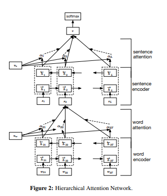
HAN was proposed by Yang et al. in 2016. Key features of HAN that differentiates itself from existing approaches to document classification are (1) it exploits the hierarchical nature of text data and (2) attention mechanism is adapted for document classification. Let’s examine what they mean and how such features are utilized for designing HAN.

Hierarchy in text

Words are composed of letters. Sentences are composed of words. Paragraphs are composed of sentences. And so on. Surely, there is a hierarchy among parts that constitute a document. Even though it seems that we understand sentences at a first glance without noticing the subtle hierarchy, our brain instinctly interprets sentences while fully considering hierarchy. Therefore, Yang et al. proposed a hierarchical structure comprising the word encoder and sentence encoder. The word encoder summarizes information on the word level and passes it onto the sentence encoder. The sentence encoder processes information on the sentence level and the output probabilities are predicted at the final layer.

Attention for classification

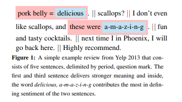
On top of hierarchy, what makes natural language more complicated is interaction between parts. Words interact with each other and also, they interact with sentences. As Steven Pinker noted, “Dog bites man” usually does not make it to the headline, but “Man bites dog” can. Furthermore, some parts are more important than others in generating the overall meaning of the document. Yang et al. have recognized this and fully incorporated in their model architecture. HAN has attention layer at both levels - i.e., word attention and sentence attention. Word attention aligns words and weighs them based on how important are they in forming the meaning of a sentence. And sentence attention aligns each sentence based on how salient they are in classifying each document. By aligning parts and attending to the right ones, HAN better understands the overall semantic structure of the document and classifies it.

In this posting, we had a brief look at hierarchical attention proposed by Yang et al. (2016). In the next posting, let’s see how they can be implemented with Pytorch.

References

Attention in Neural Networks - 14. Various attention mechanisms (3)

|

Attention Mechanism in Neural Networks - 14. Various attention mechanisms (3)

So far, we looked into and implemented scoring functions outlined by Luong et al. (2015). In this posting, let’s have a look at local attention that was proposed in the same paper.

Local attention

As mentioned in previous postings, local attention differs from global attention in that it attends to local inputs that are in the vicinity of the aligned position. There are two methods that are suggested to find the aligned position - i.e., monotonic alignment (local-m) and predictive alignment (local-p). Though the mathematical details and implementation differ, motivations and intuition behind the two are largely similar. Here, let’s examine local-m, which is simpler and more intuitive.

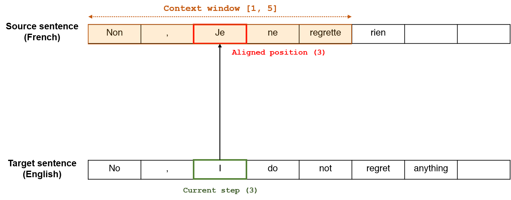
Below diagram illustrates an example of applying local-m to a real-world task of translating a French (source) sentence to an English (target) sentence. Consider translating a french sentence “Non, Je ne regrette rien”, which was also a soundtrack of the movie inception. A correct translation is “No, I do not regret anything” in English.

Let us set $D = 2$, which can be empirically selected by a developer. Consider the third step of the target sentence, where we have the word “I”. Since for local-m, we regard $p_t = t$, the aligned position is also 3, which has the word “Je” in the source sentence. This is also common-sensical since the direct translation of the French word “Je” is “I”. And since we set $D = 2$, the context window is $[1, 5]$, which comprises the words “Non, Je ne regrette”. Therefore, the decoder at the third step attends to that part of the source sentence for alignment. Then, the same scoring and normalization procedure can be applied as global attention we investigated so far.

Pytorch implementation of local-m

Now, let’s try implementing local-m with Pytorch. As we can apply the same scoring and normalization procedure, we do not need to convert the source code for the encoder and decoder that we implemented before. The only part that we need to modify is the training process to find the context window for each step in the target. One approach that we can take is set the window size $D$ and select surrounding encoder outputs at each step. The base case would be setting $[p_t-D, p_t+D]$ to include $2D+1$ encoder states.

enc_outputs_selected = enc_outputs[l-WINDOW_SIZE:l+WINDOW_SIZE+1]

However, there are edge cases that we should meticulously attend to. There are two edge cases at (1) the start of the sentence and (2) the end of the sentence, where we cannot select surrounding $2D+1$ steps. For instance, at the French-English translation example above, we cannot set the full context window of length five for the first and second target words (“Non” and ”,”). So, let’s add if-elif-else to fully consider both base and edge cases.

for l in range(target.size(0)):
  if l < WINDOW_SIZE:
    enc_outputs_selected = enc_outputs[:l+WINDOW_SIZE+1]
  elif l > target.size(0) - WINDOW_SIZE - 1:
    enc_outputs_selected = enc_outputs[l-WINDOW_SIZE:]
  else:
    enc_outputs_selected = enc_outputs[l-WINDOW_SIZE:l+WINDOW_SIZE+1]

Training local attention

Below is the complete code for training local attention models. Also note that we have to define an additional hyperparameter WINDOW_SIZE that denotes the size of the context window ($D$).

%%time
encoder_opt = torch.optim.Adam(encoder.parameters(), lr = 0.01)
decoder_opt = torch.optim.Adam(decoder.parameters(), lr = 0.01)
criterion = nn.NLLLoss()
loss = []
weights = []

for i in tqdm(range(NUM_EPOCHS)):
  for j in range(len(eng_sentences)):
    current_weights = []
    source, target = eng_sentences[j], deu_sentences[j]
    source = torch.tensor(source, dtype = torch.long).view(-1, 1).to(DEVICE)
    target = torch.tensor(target, dtype = torch.long).view(-1, 1).to(DEVICE)

    current_loss = 0
    h0 = torch.zeros(1, 1, encoder.hidden_size).to(DEVICE)

    encoder_opt.zero_grad()
    decoder_opt.zero_grad()

    enc_outputs = torch.zeros(MAX_SENT_LEN, encoder.hidden_size).to(DEVICE)
    for k in range(source.size(0)):
      _, h0 = encoder(source[k].unsqueeze(0), h0)
      enc_outputs[k] = h0.squeeze()
    
    # monotonic alignment
    dec_input = torch.tensor([[deu_words.index("<sos>")]]).to(DEVICE)
    for l in range(target.size(0)):
      if l < WINDOW_SIZE:
        enc_outputs_selected = enc_outputs[:l+WINDOW_SIZE+1]
      elif l > target.size(0) - WINDOW_SIZE - 1:
        enc_outputs_selected = enc_outputs[l-WINDOW_SIZE:]
      else:
        enc_outputs_selected = enc_outputs[l-WINDOW_SIZE:l+WINDOW_SIZE+1]

      out, h0, w = decoder(dec_input, h0, enc_outputs_selected)
      _, max_idx = out.topk(1)
      dec_input = max_idx.squeeze().detach()
      current_loss += criterion(out, target[l])
      if dec_input.item() == deu_words.index("<eos>"):
        break

    current_loss.backward(retain_graph=True)
    encoder_opt.step()
    decoder_opt.step()
    # weights.append(current_weights)

  loss.append(current_loss.item()/(j+1))

In this posting, we implemented local attention proposed by Luong et al. (2015). Thank you for reading.

References

Attention in Neural Networks - 13. Various attention mechanisms (2)

|

Attention Mechanism in Neural Networks - 13. Various attention mechanisms (2)

In the previous posting, we saw various attention methods explained by Luong et al. (2015). In this posting, let’s try implemeting differnt scoring functions with Pytorch.

Simplified concat (additive)

So far, we have implemented the scoring function as a simplified version of the concat function. Concat function, also known as additive function, was initially proposed by Bahdahanu et al. (2015). The concat function concatenates the source and target hidden states ($h_t, \bar{h_s}$), followed by a multiplication by the matrix $W_a$. Then, the multiplied result is passed onto a tangent hyperbolic activation ($tanh$) and then a dot product with another parameter $v_a^{T}$. However, we ommitted the tangent hyperbolic activation and parameter $v_a^{T}$ so far for simplicity. Therefore, what we have been implementing was, in mathematical formula:

\begin{equation} score(h_t, \bar{h_s}) = v_a^{T}tanh(W_a[h_t;\bar{h_s}]) \end{equation}

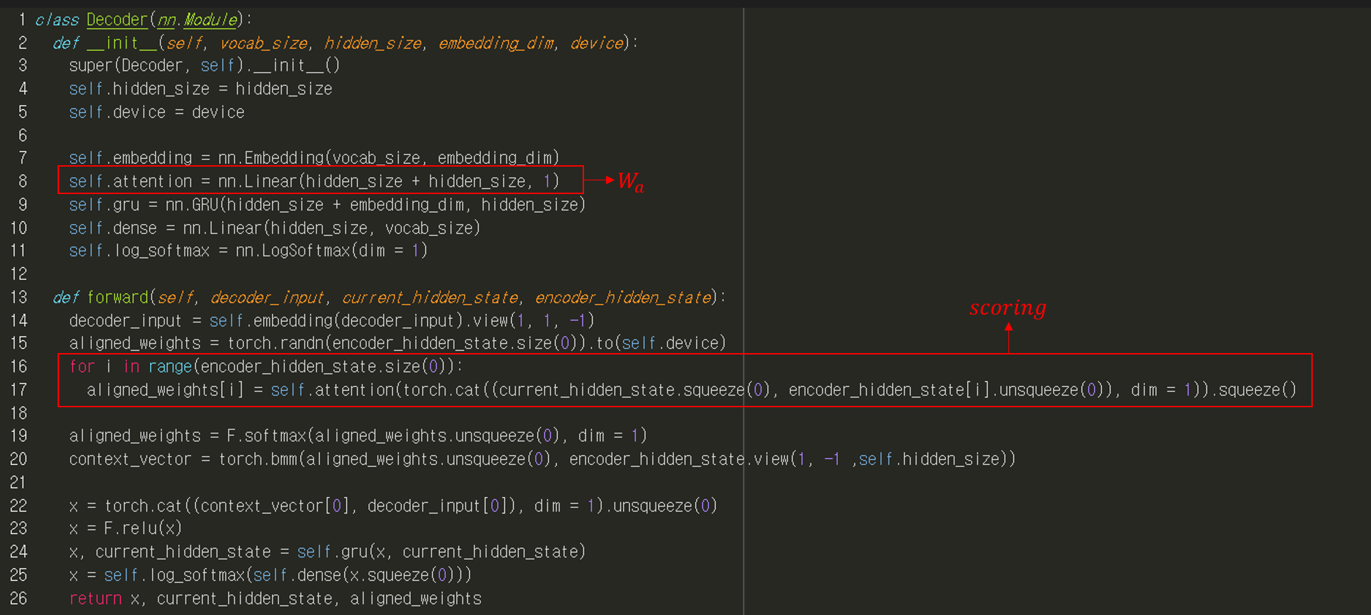
In Pytorch, it was implemented as below. Below is step-by-step procedure of the scoring operation.

  • torch.cat() function concatenates source and target states
  • self.attention layer multiplies W_a and the concatenated states
  • for loop iterates over each step in the encoder
  • F.softmax() function normalizes scored weights.

Concat (additive)

For the concat function, not the simplified one, we just need to add an activation and dot product with $v_a^{T}$. Therefore, in the init() function of the decoder class, we define another parameter vt for $v_a^{T}$. This parameter will be jointly trained with other parameters in the network.

self.attention = nn.Linear(hidden_size + hidden_size, hidden_size)
self.vt = nn.Parameter(torch.FloatTensor(1, hidden_size))

In the forward function, we just need to add few things. F.tanh() function will apply the tangent hyperbolic activation over matrix-multiplied outputs. Then, torch.dot() function will perform the dot product of the parameter and the intermediate output.

for i in range(encoder_hidden_state.size(0)):
    w = F.tanh(self.attention(torch.cat((current_hidden_state.squeeze(0), encoder_hidden_state[i].unsqueeze(0)), dim = 1)))
    aligned_weights[i] = torch.dot(self.vt.squeeze(), w.squeeze())

General

The general scoring function is simpler than the concat function. Instead of concatenating $h_t$ and $\bar{h_s}$ and multiplying with the matrix $W_a$, the general function multiplies $h_t$, $W_a$, and $\bar{h_s}$

\begin{equation} score(h_t, \bar{h_s}) = h_t^{T}W_a\bar{h_s} \end{equation}

Therefore, for the general function we only need the dense layer that performs matrix multiplication by $W_a$. However, note that self.attention layer here has the input size of hidden_size, instead of hidden_size * 2 as in the concat function. This difference in input dimension arises because the two hidden states are not concatenated in the general scoring function. Therefore, the input size of the general function is equal to the hidden size of \bar{h_s}.

self.attention = nn.Linear(hidden_size, hidden_size)

The computation of weights are also simpler. The source hidden states (encoder_hidden_state) are multiplied with $W_a$ by self.attention() and then dot-producted with the target hidden state (current_hidden_state).

aligned_weights[i] = torch.dot(current_hidden_state.squeeze(), self.attention(encoder_hidden_state[i].unsqueeze(0)).squeeze())

Dot

The dot scoring function is the most straightforward one. It is consisted of just a dot product of two hidden states ($h_t, \bar{h_s}$). No additional parameters to be defined and learned. We just need to multiply them with torch.dot() function to calculate the weights.

aligned_weights[i] = torch.dot(current_hidden_state.squeeze(), encoder_hidden_state[i].squeeze())  

Decoder - putting it altogether

It would be cumbersome to define a different decoder class everytime for a different scoring function. Therefore, we manage is with an additional parameter scoring that denotes the type of scoring function that is going to be used. Below is the decoder class that takes into account choosing different scoring functions.

class Decoder(nn.Module):
  def __init__(self, vocab_size, hidden_size, embedding_dim, scoring, device):
    super(Decoder, self).__init__()
    self.hidden_size = hidden_size
    self.device = device
    self.scoring = scoring

    self.embedding = nn.Embedding(vocab_size, embedding_dim)

    if scoring == "concat":
      self.attention = nn.Linear(hidden_size + hidden_size, hidden_size)
      self.vt = nn.Parameter(torch.FloatTensor(1, hidden_size))
    elif scoring == "general":
      self.attention = nn.Linear(hidden_size, hidden_size)
    self.gru = nn.GRU(hidden_size + embedding_dim, hidden_size)
    self.dense = nn.Linear(hidden_size, vocab_size)
    self.log_softmax = nn.LogSoftmax(dim = 1)
  
  def forward(self, decoder_input, current_hidden_state, encoder_hidden_state):
    decoder_input = self.embedding(decoder_input).view(1, 1, -1)
    aligned_weights = torch.randn(encoder_hidden_state.size(0)).to(self.device)

    if self.scoring == "concat":
      for i in range(encoder_hidden_state.size(0)):
        w = F.tanh(self.attention(torch.cat((current_hidden_state.squeeze(0), encoder_hidden_state[i].unsqueeze(0)), dim = 1)))
        aligned_weights[i] = torch.dot(self.vt.squeeze(), w.squeeze())
  
    elif self.scoring == "general":
      for i in range(encoder_hidden_state.size(0)):
        aligned_weights[i] = torch.dot(current_hidden_state.squeeze(), self.attention(encoder_hidden_state[i].unsqueeze(0)).squeeze())

    elif self.scoring == "dot":
      for i in range(encoder_hidden_state.size(0)):
        aligned_weights[i] = torch.dot(current_hidden_state.squeeze(), encoder_hidden_state[i].squeeze())    

    aligned_weights = F.softmax(aligned_weights.unsqueeze(0), dim = 1)
    context_vector = torch.bmm(aligned_weights.unsqueeze(0), encoder_hidden_state.view(1, -1 ,self.hidden_size))
    
    x = torch.cat((context_vector[0], decoder_input[0]), dim = 1).unsqueeze(0)
    x = F.relu(x)
    x, current_hidden_state = self.gru(x, current_hidden_state)
    x = self.log_softmax(self.dense(x.squeeze(0)))
    return x, current_hidden_state, aligned_weights

In this posting, we tried implementing various scoring function delineated in Luong et al. (2015). So far, we implemented just global attention mechanism. In the following postings, let’s have a look into how local attention can be implemented.

References